Evaluating SNR Performance of FMFB Demodulators at High CNR

The previous article in this series explored the essential workings of the FMFB circuit, particularly its approach to FM demodulation and its capability to reduce the noise threshold. Building on that foundation, this article calculates the output SNR of the FMFB demodulator at high carrier-to-noise ratio (CNR) values. We’ll demonstrate that, despite the FMFB’s ability to reduce the noise threshold, it has no effect on output SNR in high-CNR conditions. In other words, the FMFB circuit achieves the same SNR as a conventional non-feedback demodulator when the input CNR is high.

 

Brief Recap of FMFB Fundamentals

Shown in Figure 1 is the basic block diagram of the FMFB demodulator.

 

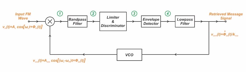
Figure 1. Functional block diagram of the FMFB demodulator.

 

Assume the input FM signal takes the form:

$$v_{in}(t) = A_c \ cos[\omega_c t + \phi_{in}(t)]$$

Equation 1

where:
A_c is the amplitude of the input FM wave
ω_c is the carrier frequency
ϕ_in(t) is the message-dependent phase term.

The mathematical analysis provided in the previous article shows that the FMFB demodulator output is given by:

$$v_{cont}(t) = \frac{\alpha}{1 + \alpha \times k_{vco}} \times \frac{d}{dt}\phi_{in}(t)$$

Equation 2

where:
⍺ is the gain factor of the conventional demodulator incorporated in the forward path
k_vco is the VCO gain factor measured in radians per second per volt (rad/sV).

Since ϕ_in(t) represents the phase of the input FM wave, it’s proportional to the integral of the message signal. Therefore, we observe that the VCO control voltage produces the output of the conventional demodulator—⍺ times the derivative of ϕ_in(t)—but attenuated by the factor 1 +⍺k_vco.

Another key effect of the feedback configuration is a reduction in the deviation ratio, specifically by a factor of 1+⍺k_vco. As a result, the required bandwidth of the IF bandpass filter in the FMFB demodulator is reduced by a factor of 1+⍺k_vco compared to a non-feedback FM demodulator. This bandwidth reduction lowers system noise and improves the FM detection threshold.

 

SNR Performance of FMFB at High Carrier-to-Noise Ratios

We understand that the FMFB demodulator reduces the noise threshold, but how does the feedback mechanism influence the output SNR under high CNR conditions? Before presenting the analysis, we’d like to share its concluding results to provide insight into what we’re discussing and what you can expect. Figure 2 compares the output SNR of the FMFB demodulator with that of a non-feedback FM demodulator.

 

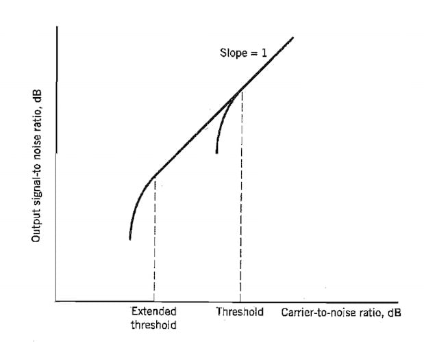
Figure 2. The FMFB demodulator reduces the threshold, but it doesn’t affect the SNR at high CNR values. Image used courtesy of Simon Haykin.

 

We observe that although the FMFB demodulator decreases the threshold, it achieves the same SNR as the conventional demodulator when the input CNR is high. This may seem counterintuitive initially, as you might anticipate a higher SNR resulting from the noise bandwidth reduction achieved by the narrowband IF bandpass filter.

For instance, the bandpass filter in the FMFB demodulator may have a bandwidth that is just one-fifth of that in a conventional demodulator. This narrower bandwidth effectively reduces the noise entering the frequency discriminator, which suggests an expected improvement in SNR. To clarify this confusion, we’ll compute the output SNR of the FMFB circuit to better understand its noise characteristics.

 

Calculating the Output Signal Power

Let’s begin by calculating the output signal power. According to the fundamentals of the FM scheme, we recognize that the input phase term ϕ_in(t) is associated with the message signal m(t) through the following relationship:

$$\phi (t) = 2 \pi k_f \int_{0}^{t} m(\tau) \ d \tau$$

Equation 3

 

where k_f is the frequency deviation constant. The FMFB demodulator output is given by:

$$v_{cont}(t) = \frac{\alpha}{1 + \alpha \times k_{vco}} \times \frac{d}{dt}\phi_{in}(t)$$

Equation 4

 

Therefore, the output signal power becomes:

$$P_{s,out} = \Big (\frac{\alpha}{1 + \alpha \times k_{vco}} \Big )^2 \times 4 \pi^2 \times k_{f}^{2} \times P_{m}$$

Equation 5

 

where P_m is the average power of the message signal. To simplify our equations, we’ll take ⍺ = 1 as an assumption for the rest of this article, which lets us rewrite the output signal power equation as:

$$P_{s,out} = \frac{1}{(1 + k_{vco})^2} \times 4 \pi^2 \times k_{f}^{2} \times P_{m}$$

Equation 6

 

Noise Transformation Through the FMFB Demodulator

For a simplified analysis of the circuit’s noise behavior, let the input signal be an unmodulated carrier: v_in(t) = A_ccos(ω_ct). Furthermore, assume a carrier bandpass filter is placed ahead of the FMFB demodulator to isolate the desired FM signal and suppress adjacent-channel and out-of-band interference. Hence, the noise entering the demodulator is narrowband noise concentrated around the carrier frequency ω_c. The total input, including both signal and noise, may be expressed as:

$$v_{in}(t) + n_{filtered}(t) = A_c cos (\omega_c t) + n_{I}(t) \ cos(\omega_c t) - n_{Q}(t) \ sin(\omega_c t)$$

Equation 7

 

where n_I(t) and n_Q(t) are the in-phase and quadrature components of the noise. The FMFB demodulator uses a VCO whose free-running frequency is ω_c-ω_IF, where ω_IF is the center frequency of the IF bandpass filter following the mixer. Therefore, the VCO output can be represented by:

$$v_{vco}(t) = A_{vco} \ cos[(\omega_c - \omega_{IF})t + \phi_{ex}(t)]$$

Equation 8

 

where ϕ_ex(t) is the excess phase of the VCO. When two sinusoidal waves are applied to a multiplier mixer, the output contains frequency components equal to both the sum and difference of the input frequencies. If we multiply the noisy input (Equation 7) by the VCO output, we obtain the following difference frequency components at the output of the mixer:

$$\frac{1}{2} \big (A_c+n_I(t) \big ) \ A_{vco} \times cos \big [\omega_{IF} t - \phi_{ex}(t) \big ] - \frac{1}{2} n_Q(t) A_{vco} \times sin \big [ \omega_{IF}t - \phi_{ex} (t) \big ]$$

Equation 9

 

Note that the IF bandpass filter centered at ω_IF permits the passage of the difference frequency components from the mixing process while blocking the sum frequency components. Therefore, we don’t need to calculate the sum frequency components.

How does the IF bandpass filter affect the difference frequency components? As these frequency components pass through the IF bandpass filter, the noise bandwidth is reduced from the carrier filter’s bandwidth B_c to that of the IF filter B_IF. To account for this effect, we’ll denote the in-phase and quadrature noise components at the IF filter output as n_I,2(t) and n_Q,2(t). Replacing n_I(t) and n_Q(t) in Equation 9 with n_I,2(t) and n_Q,2(t), the noisy signal at the output of the IF filter (node 2) is given by:

$$v_{2}(t) = \frac{1}{2} \big (A_c+n_{I,2}(t) \big ) \ A_{vco} \times cos \big [\omega_{IF} t - \phi_{ex}(t) \big ] - \frac{1}{2} n_{Q,2}(t) \ A_{vco} \times sin \big [ \omega_{IF}t - \phi_{ex}(t) \big ]$$

Equation 10

 

If the original noise components (n_I(t) and n_Q(t)) have a two-sided power spectral density of N₀ Watts/Hz over -B_c/2B_c/2, then the filtered components (n_I,2(t) and n_Q,2(t)) retain the same spectral density N₀, but over the reduced bandwidth -B_IF/2B_IF/2. This results in a reduction of the average noise power by a factor of B_c/B_IF relative to the noise power at the output of the carrier filter.

Equation 10 can be simplified into a single sinusoidal function using amplitude-phase form. Specifically, the expression A cos(x) + B sin(x) equals Rcos(x - θ) where R and θ are given by:

$$R = \sqrt{A^2+B^2} \quad \text{and} \quad \theta = \tan^{-1}\Big(\frac{B}{A}\Big)$$

Equation 11

 

Applying this identity, the signal at node 2 (shown in Equation 10) can be rewritten as:

$$v_2(t) = R\cos\big[\omega_{IF}t - \phi_{ex}(t) + \theta\big]$$

Equation 12

 

where the phase term θ is given by:

$$\theta = \tan^{-1}\Big(\frac{\frac{1}{2}n_{Q,2}(t)A_{vco}}{\frac{1}{2}(A_c+n_{I,2}(t))A_{vco}}\Big) = \tan^{-1}\Big(\frac{n_{Q,2}(t)}{A_c+n_{I,2}(t)}\Big)$$

Equation 13

 

The amplitude term R in Equation 12 is of no interest to us because the limiter incorporated in the forward path of the FMFB circuit removes all variations in the envelope. When the CNR is high, i.e. the noise components n_I,2(t) and n_Q,2(t) are much smaller than the carrier amplitude A_c, we simplify the phase term θ to:

$$\theta \approx \frac{n_{Q,2}(t)}{A_c}$$

Equation 14

 

The phase term θ indicates the angular modulation of the input FM waveform due to the presence of noise. Using Equation 2, the output of the FMFB demodulator due to θ is given by:

$$v_{cont}(t) = \frac{1}{A_c(1+k_{vco})} \times \frac{d}{dt}[n_{Q,2}(t)]$$

Equation 15

 

Note that ⍺ = 1 is assumed in the derivation of the above equation. If you find it difficult to grasp how we arrived at Equation 15, we suggest revisiting the previous article in this series.

 

Calculating Average Output Noise Power

Equation 15 shows how the input noise transforms as it travels through the FMFB demodulator. According to this equation, the output noise is proportional to the time derivative of the quadrature noise component n_Q,2(t). In the frequency domain, differentiation corresponds to multiplication by jω. Therefore, the power spectral density of the output noise is:

$$S_n(\omega) = \Big|\frac{1}{A_c(1+k_{vco})} \times j\omega\Big|^2 \times S_{n_Q}(\omega) = \Big(\frac{\omega}{A_c(1+k_{vco})}\Big)^2 \times N_0$$

Equation 16

 

where S_nQ(ω) denotes the power spectral density of the quadrature noise component. Note that if the white noise at the input has a two-sided spectral density of N₀/2, the in-phase and quadrature noise components will have a spectral density of N₀ around DC, as illustrated in Figure 3 below.

 

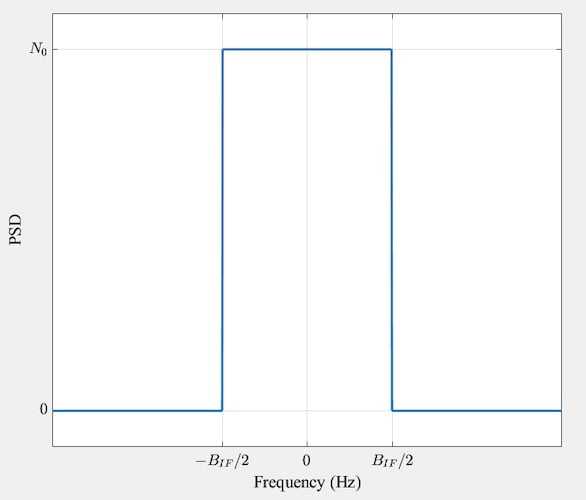
Figure 3. The power spectral density of the quadrature noise component.

 

Note that the bandwidth of the quadrature noise component n_Q,2(t) is determined by the IF bandpass filter. As outlined in Equation 16 and illustrated in Figure 4 below, the power spectral density of the output noise exhibits a parabolic shape due to the differentiating nature of the FM discriminator.

 

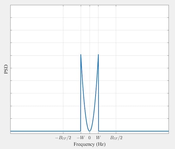
Figure 4. The power spectral density of noise at the output of the lowpass filter.

 

If the message bandwidth is W hertz, we usually use a lowpass filter with bandwidth W at the discriminator output to minimize the noise. Therefore, the power spectral density of the output noise spans from -W to W hertz, as illustrated in the figure above. The average output noise power is obtained by taking the integral of the output power spectral density (Equation 13) over -2π×W to +2π×W:

$$P_{n,out} = \frac{1}{2\pi}\int_{-2\pi W}^{+2\pi W}\Big(\frac{\omega}{A_c(1+k_{vco})}\Big)^2 \times N_0\,d\omega = \frac{1}{(1+k_{vco})^2} \times \frac{8\pi^2 \times N_0 W^3}{3A_c^2}$$

Equation 17

 

Deriving the FMFB Demodulator SNR

Using the signal and noise power expressions (Equations 6 and 17), we can now determine the SNR of the FMFB demodulator:

$$SNR_{out} = \frac{P_{s,out}}{P_{n,out}} = \frac{\Big(\frac{1}{1+k_{vco}}\Big)^2 \times 4\pi^2 \times k_f^2 \times P_m}{\Big(\frac{1}{1+k_{vco}}\Big)^2 \times \frac{8\pi^2 \times N_0 W^3}{3A_c^2}} = \frac{3A_c^2 \times k_f^2 \times P_m}{2 \times N_0 W^3}$$

Equation 18

 

Interestingly, the SNR relation for the FMFB demodulator is the same as that for the traditional demodulator, which operates without feedback (compare Equation 18 above with Equation 17 of this article).

 

Why Is Threshold Improved But Not SNR?

When comparing the expressions for output signal and noise power (Equations 6 and 17) with those of the non-feedback demodulator (Equations 4 and 16 of this article), you will find that the FMFB demodulator alters both the signal and noise components by the same gain factor, specifically 1/(1+k_vco). That’s why the feedback doesn’t alter the SNR.

Note that although the narrowband IF filter reduces the bandwidth within the loop, the noise bandwidth is ultimately determined by the lowpass filter following the demodulator. Since both the FMFB and conventional demodulators utilize lowpass filters with the same bandwidth, the reduction in the IF filter bandwidth doesn’t enhance the SNR.

However, the narrowband IF filter reduces the noise that enters the discriminator. If you’ve read our article on the threshold effect in FM systems, you may remember that when the carrier and noise amplitudes at the input of the discriminator are comparable, noise fluctuations can occasionally cause the noisy input vector to sweep around the origin. As illustrated in Figure 5 below, this results in a 2π-radian phase increase or decrease in the noisy input vector, leading to noticeable spikes in the FM demodulator output.

 

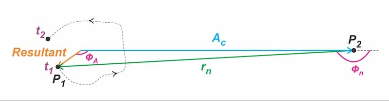
Figure 5. Phasor diagram representation of the noisy FM wave when the CNR is low.

 

Wrapping Up

In this article, we derived the output SNR of the FMFB demodulator and showed that, despite reducing the noise threshold, the feedback configuration provides no SNR improvement over a conventional non-feedback demodulator at high CNR. The FMFB circuit instead lowers the threshold by reducing the noise reaching the discriminator, thereby delaying the onset of threshold effects such as phase wrapping in the noisy input vector. In the next article, we’ll use solved examples to illustrate typical threshold improvements provided by the FMFB configuration, then examine the PLL-based FM demodulator and its own approach to threshold reduction.