SNR Analysis of FM Modulation with Arbitrary Message Signals

Previously, we examined how additive white Gaussian noise impacts FM signals during tone modulation, where the message was a single-frequency sinusoid. Building on that foundation, this article extends the analysis to derive the general signal-to-noise ratio (SNR) expression for FM modulation with arbitrary message signals.

We also revisit the simplifications made in the previous article to clarify how they shaped the tone-modulated analysis. FM noise analysis can get fairly complex, but we’ll walk through it step by step to keep things as clear and digestible as possible.

 

FM Demodulator Model Used in SNR Derivation

Shown in Figure 1 is the FM demodulator model typically used for noise analysis.

 

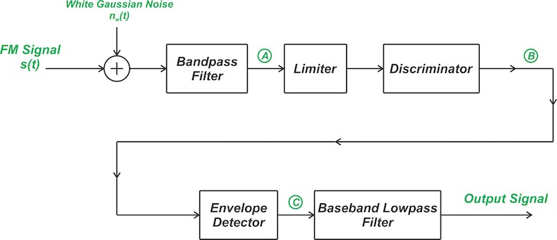
Figure 1. An FM receiver processing a noisy FM wave.

 

Using the above model, we analyze the transformation of both the input signal and noise components as they traverse various stages of the FM demodulator. Subsequently, we compute the output signal-to-noise ratio (SNR) to evaluate the performance quality of the FM receiver.

 

Calculating the Output Signal Power

The FM wave applied to the demodulator is described by:

$$s(t)= A_c \ cos \Big [ 2 \pi f_c t + \phi(t) \Big ]$$

Equation 1.

 

where A_c is the carrier amplitude, and f_c is its frequency. The phase term ϕ(t) is proportional to the integral of the message signal m(t), as illustrated in the equation below:

$$\phi (t) = 2 \pi k_f \int_{0}^{t} m(\tau) d \tau$$

Equation 2.

 

where k_f is the frequency deviation constant. To calculate the output signal power, we apply the noise-free FM wave defined in Equation 1 to our demodulator model and determine the output signal power. The FM demodulator produces the derivative of the phase term ϕ(t). Therefore, the output signal is:

$$v_o(t) = \frac{d}{dt} \phi(t) = 2 \pi k_{f} \times m(t)$$

Equation 3.

 

The output signal power is obtained as:

$$P_{s,out} = 4 \pi^2 \times k_{f}^{2} \times P_{m}$$

Equation 4.

 

where P_m is the average power of the message signal. Let’s put the equation we just derived to work and verify the result from our earlier tone-modulated FM case. When the message is a simple sinusoid, m(t) = A_mcos(2πf_mt), the average power of the message is P_m = A_m²/2, producing:

$$P_{s,out} = 4 \pi^2 \times k_{f}^{2} \times \frac{A_m^2}{2} = 4 \pi^2 \times \frac{\beta^2 f_{m}^2}{2} = \frac{\beta^2 \omega_{m}^2}{2}$$

Equation 5.

 

where the definition of the modulation index β reproduced below is used to simplify the result:

$$\beta = \frac{k_f A_m}{ f_m}$$

Equation 6.

 

You can verify that Equation 5 is consistent with the results of the previous article. Equation 4 suggests that the message power P_m should emerge in the final SNR formulation.

 

Noise Transformation Through the Demodulator

In the presence of noise, the total input applied to the demodulator is s(t)+n_w(t), where n_w(t) denotes additive white Gaussian noise with a zero mean and a double-sided power spectral density of N₀/2 Watts/Hz. At the output of the bandpass filter (node A in Figure 1), we have a filtered noise process n_filtered(t) that can be expressed in terms of its in-phase and quadrature components, n_I(t) and n_Q(t). Therefore, the noisy signal applied to the limiter is:

$$s(t) + n_{filtered}(t) = A_c cos \Big [ 2 \pi f_c t + \phi(t) \Big ] + n_{I}(t) \ cos(2 \pi f_c t) - n_{Q}(t) \ sin(2 \pi f_c t)$$

Equation 7.

 

To conduct a precise analysis, we can employ the phasor representation of the three components in the preceding equation to characterize the composite signal fed into the limiter. The output corresponds to the time derivative of this composite signal, which is evidently influenced by noise. Given the complexity of this approach, we commonly introduce simplifying assumptions to facilitate tractable analysis.

 

Phasor Representation for φ(t) = 0

As discussed in the previous article, we computed the output noise power under the assumption that no signal was present, i.e., ϕ(t) = 0. We now revisit that analysis using the phasor representation to build familiarity with this method before extending it to the more general case where ϕ(t) is non-zero. Assuming a carrier with no modulation and expressing the noise components in polar coordinates, Equation 7 simplifies to:

$$s(t) + n_{filtered}(t) = A_c cos (2 \pi f_c t) + r_{n}(t) \ cos \big (2 \pi f_c t + \phi_{n}(t) \big )$$

Equation 8.

 

where r_n(t) and ϕ_n(t) are, respectively, the envelope and instantaneous phase of the noise. According to probability theory, the envelope r_n(t) of the noise follows a Rayleigh distribution, while its instantaneous phase ϕ_n(t) is uniformly distributed over 2π radians. We’ll see how the uniformity of the phase distribution plays a key role in the next section. Shown below is the phasor form of the vector summation in Equation 8.

 

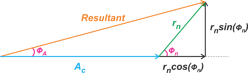
Figure 2. Phasor diagram for unmodulated carrier wave plus noise.

 

The FM demodulator produces the derivative of the resultant vector’s phase angle ϕ_A. Thus, to understand the impact of noise, it’s necessary to derive an expression for ϕ_A. Assuming that the noise components r_ncos(ϕ_n) and r_nsin(ϕ_n) are much smaller than the carrier amplitude A_c, we approximate the resultant vector’s phase as:

$$\phi_{A}(t) = tan^{-1} \Big( \frac{r_{n} sin(\phi_{n}))}{A_c + r_{n} cos(\phi_{n}))} \Big) \approx tan^{-1} \Big( \frac{r_{n} sin(\phi_{n}))}{A_c} \Big) \approx \frac{r_{n} sin(\phi_{n}))}{A_c}$$

Equation 9.

 

The term r_nsin(ϕ_n) is equal to the quadrature component of the noise n_Q(t), hence, ϕ_A(t) becomes:

$$\phi_{A}(t) \approx \frac{n_{Q}(t)}{A_c}$$

Equation 10.

 

Since the demodulator produces the derivative of ϕ_A(t), the noise component at the output (node C in Figure 1) is:

$$n_{C}(t) \approx \frac{1}{A_c} \times \frac{d}{dt}n_{Q}(t)$$

Equation 11.

 

Consistent with the results of the previous article, Equation 11 shows that the additive noise appearing at the output of the demodulator depends on the carrier amplitude and the quadrature component of noise. Moreover, the output noise appears independent of the message signal ϕ(t). However, it remains to be seen whether this outcome stems from assuming ϕ(t) = 0, or if it holds more generally. This question will be addressed in the following section.

 

Phasor Representation With Non-Zero ϕ(t)

Without the simplifying assumption of ϕ(t) = 0, the carrier vector in Equation 8 acquires an initial phase of ϕ(t), which varies with the message as defined by Equation 2. In this case, we obtain the phasor diagram shown below.

 

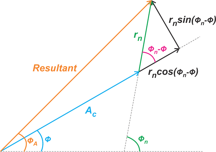
Figure 3. The phasor diagram of the noisy FM wave when ϕ(t) is non-zero.

 

Although the phasor diagram may initially appear complex, it simplifies upon closer inspection. To understand the construction of the phasor diagram, note that:

1. The carrier phasor (blue) has a phase angle of ϕ(t)
2. The noise vector (green) has a phase angle of ϕ_n(t)
3. The phase angle of the resultant vector (orange) is denoted by ϕ_A(t). The objective is to compute the resultant phase angle ϕ_A(t).

 

By applying elementary geometric principles, the angle formed between the noise vector r_n(t) and the continuation of the carrier vector is clearly ϕ_n(t) - ϕ(t). Now that we know the angle, we break down r_n(t) into two components: one aligned with the carrier vector and the other orthogonal to it. From the phasor diagram, it’s straightforward to determine the resultant phase angle:

$$\phi_{A}(t) = \phi(t) + \tan^{-1} \bigg ( \frac{r_{n}sin \big ( \phi_n(t)-\phi(t) \big )}{A_{c} + r_{n}cos \big ( \phi_n(t) - \phi(t) \big )} \bigg)$$

Equation 12.

 

Assuming that the noise components are significantly smaller than the carrier amplitude most of the time, the above equation can be approximated as:

$$\begin{eqnarray} \phi_{A}(t) &\approx& \phi(t) + \tan^{-1} \bigg ( \frac{r_{n}\sin \big ( \phi_n(t)-\phi(t) \big )}{A_{c}} \bigg ) \\ &\approx& \phi(t) + \frac{r_{n}}{A_{c}} \times \sin \big ( \phi_n(t) - \phi(t) \big ) \end{eqnarray}$$

Equation 13.

 

This is the phase angle applied to the limiter in Figure 1. We know that the demodulator produces the derivative of ϕ_A(t). The derivative of the first term on the right-hand side of the above equation corresponds to the desired signal (refer to Equation 2), whereas the derivative of the second term introduces unwanted noise at the output. Accordingly, the noise component observed at the demodulator output (node C) becomes:

$$n_{C}(t) = \frac{1}{A_c} \times \frac{d}{dt} \bigg ( r_{n} \times sin \big ( \phi_n(t)-\phi(t) \big ) \bigg )$$

Equation 14.

 

The noise equation still remains relatively complex and further simplification is necessary before we can derive the SNR expression. We mentioned earlier that the phase ϕ_n(t) is uniformly distributed over 2π radians. What if the phase ϕ_n(t) - ϕ(t) were also uniformly distributed over 2π radians? In that case, the noise term defined in Equation 14 would be independent of the message signal, and in a statistical sense, we could substitute ϕ_n(t) - ϕ(t) with ϕ_n(t).

Since ϕ_n(t) has a uniform distribution over 2π radians, in the sense of ensemble averages, ϕ_n(t) - ϕ(t) differs from ϕ_n(t) only by a shift of the mean value. Therefore, we approximate Equation 14 as:

$$n_{C}(t) = \frac{1}{A_c} \times \frac{d}{dt} \bigg ( r_{n} \times sin \big ( \phi_n(t) \big ) \bigg ) = \frac{1}{A_c} \times \frac{d }{dt}n_{Q}(t)$$

Equation 15.

 

A comparison of Equations 11 and 15 reveals that the output noise expression remains unchanged, whether we assume ϕ(t) = 0 from the outset or retain it and later apply the mentioned simplifying assumptions. Therefore, when the noise components are significantly smaller than the carrier, the output noise of the FM system is independent of the message signal ϕ(t).

Before moving forward, if the preceding rationale for replacing ϕ_n(t) - ϕ(t) with ϕ_n(t) doesn’t fully convince you, I suggest consulting Section 6.2 of Fundamentals of Communication Systems by John G. Proakis, where you'll find an alternative, more detailed explanation.

 

Calculating Average Output Noise Power

Because the noise expression remains unchanged, we directly apply the result from the previous article to obtain the average output noise power. The noise spectrum has a parabolic shape due to the differentiating action of the FM discriminator. For a message bandwidth of W hertz, the average output noise power is obtained by taking the integral of the corresponding power spectral density over -2π × W to +2π × W:

$$P_{n,out} = \frac{1}{2 \pi} \int_{-2 \pi W}^{+2 \pi W} \frac{N_O}{A_c^2}\times \omega^2 \ d \omega = \frac{8 \pi^2 \times N_O W^3}{3 A_c^2}$$

Equation 16.

 

Calculating the Output SNR

Using the signal and noise power expressions (Equations 4 and 16), we now determine the SNR of the FM scheme:

$$SNR_{out} = \frac{P_{s,out}}{P_{n, out}} = \frac{4 \pi^2 \times k_{f}^{2} \times P_{m}}{\frac{8 \pi^2 \times N_O W^3}{3 A_c^2}} = \frac{3 A_c^2 \times k_{f}^{2} \times P_{m}}{2 \times N_O W^3}$$

Equation 17.

 

The average power in the modulated signal is A_c²/2 whereas the average input noise power over the message bandwidth is WN₀. Therefore, the baseband SNR is:

$$\gamma = \frac{A_c^2}{2 N_O W}$$

Equation 18.

 

Dividing the output SNR by the baseband SNR, we get a figure of merit for the noise performance of the FM scheme:

$$\frac{SNR_{out}}{\gamma} = \frac{ 3k_{f}^{2} \times P_{m} }{W^2}$$

Equation 19.

 

An Alternative Formulation of the SNR Equation

A more useful form of the SNR equation can be obtained by noting that the deviation ratio D in FM is given by:

$$D = \frac{k_f}{W} \times Max(|m(t)|)$$

Equation 20.

 

Combining Equations 19 and 20, we have:

$$\frac{SNR_{out}}{\gamma} = 3 \times D^2 \times \underbrace{\frac{P_{m}}{ \big ( Max(|m(t)|) \big )^2}}_{\text{Power of Normalized Message}}$$

Equation 21.

 

This shows that the noise figure of merit of the FM system is a quadratic function of the deviation ratio. In wideband FM, the transmission bandwidth scales approximately with the deviation ratio D. Consequently, increasing the deviation ratio D leads to an improvement in the received SNR, but at the cost of consuming more bandwidth. This reflects a fundamental trade-off in FM systems: bandwidth is exchanged for enhanced noise performance.

Before moving forward, note that the term indicated by the underbrace in the preceding equation corresponds to the average-to-peak power ratio of the message signal, or equivalently, the normalized message power. Let’s now look at an example to solidify some of the above concepts.

 

Example: Noise-Bandwidth Trade-off in Commercial FM Broadcasting

Consider the typical modulation parameters for commercial FM broadcasting, where the highest audio frequency is commonly assumed to be W = 15 kHz, and the deviation ratio is D = 5. Calculate the noise figure of merit for this system assuming that the power of the normalized message is 0.5. Use Carson’s rule to estimate the FM signal bandwidth.

 

Solution:

By inserting the given values into Equation 21, we obtain:

$$\frac{SNR_{out}}{\gamma} = 3 \times 5^2 \times 0.5 = 37.5$$

Equation 22.

 

This means that the noise performance of the broadcast FM system is about 10log(37.5) ≈ 16 dB better than analog baseband transmission. In other words, with all parameters being equal, a 1 W FM system provides the same SNR performance as a 37.5 W baseband system. The improvement in SNR, or equivalently the reduction in transmitted power, comes at the expense of increased transmission bandwidth. Applying Carson’s rule, the FM signal bandwidth is:

$$BW = 2(D+1)W = 2(5+1) \times 15 \ kHz = 180 \ kHz$$

Equation 23.

 

which is 12 times wider than the message bandwidth.

 

Final Thoughts

In this article, we derived the general SNR expression for FM modulation with arbitrary message signals. We saw that increasing the deviation ratio D enhances the received SNR, albeit at the expense of greater bandwidth consumption. This illustrates a core principle in FM system design: a trade-off between spectral efficiency and noise resilience.

While this article focused on deriving the general SNR expression analytically, the next article will visualize how signal and noise power vary with the deviation ratio for FM systems carrying arbitrary message signals.