Facebook
 Google
 GitHub
 Linkedin
FM-to-AM Conversion Using the Foster-Seeley Discriminator
Learn how the Foster-Seeley discriminator, a classic analog circuit for FM demodulation, achieves its superior linearity.
In the previous article, we learned how slope detectors for FM demodulation transform frequency deviation into amplitude deviation. Following this conversion from FM to AM, the message signal is retrieved by an envelope detector. In this article, we'll explore another classic FM demodulation circuit: the Foster-Seeley discriminator, which is shown in Figure 1.

Figure 1. The Foster-Seeley discriminator.
For frequencies above resonance, the output voltage of this circuit is positive. For frequencies below resonance, the output voltage is negative. The frequency response of the Foster-Seeley discriminator can be seen in Figure 2.

Figure 2. Typical frequency response of the Foster-Seeley discriminator.
How the Foster-Seeley discriminator achieves this response might not be immediately clear from its schematic. To clarify, we'll examine the operation of the circuit's key components. We'll then build on what we've learned to explain the overall circuit's functionality.
Let's start by exploring the behavior of a series RLC circuit near its resonant frequency, with a focus on the phase shift it introduces.
Understanding an RLC Circuit's Phase Shift
Figure 3 shows the parallel connection of L2 and C2 from the above schematic. R2 is added to represent the parasitic resistance of L2.

Figure 3. An example of an RLC circuit.
For the purpose of this discussion, let's assume the following values:
L2 = 10 μH
R2 = 100 Ω
C2 = 25.33029 pF.
This results in a resonant frequency of 10 MHz, as calculated below:
$$f_r ~=~ \frac{1}{2 \pi \sqrt{L_2 C_2}}~=~\frac{1}{2 \pi \sqrt{10 ~\times~ 10^{-6} ~\times~ 25.33029 ~\times~ 10^{-12}}} ~=~ 10 \ \text{MHz}$$
Equation 1.
We now apply a 10 MHz sinusoidal input and take the voltage across the capacitor as the output. Figure 4 shows the result from an LTspice simulation.

Figure 4. Input voltage (blue) and output voltage (red) for a 10 MHz signal.
The input and output waveforms' relative positions along the time axis clearly indicate that the output is –90 degrees out of phase with the input. This means the circuit introduces a –90 degree phase shift at the resonant frequency. While we could certainly confirm this mathematically, in this article we'll use simulation results to gain perspective without delving into the mathematical proof.
If we increase the input frequency to 10.2 MHz, we obtain the waveforms in Figure 5.

Figure 5. Input voltage (blue) and output voltage (red) for a 10.2 MHz signal.
For frequencies above the resonant frequency, the absolute value of the phase shift is greater than –90 degrees. Figure 6 displays the waveforms at 9.8 MHz, which is slightly below the resonant frequency.

Figure 6. Input voltage (blue) and output voltage (red) for a 9.8 MHz signal.
Below the resonant frequency, the absolute value of the phase shift is smaller than –90 degrees. The same results can be obtained by using an AC analysis, the results of which are shown in Figure 7.

Figure 7. The RLC circuit's frequency response: magnitude (top) and phase (bottom).
Within a narrow frequency band around the resonant frequency, the magnitude response remains nearly constant while the phase shift varies approximately linearly with frequency. This frequency-sensitive phase shift is employed in the Foster-Seeley discriminator to demodulate FM waves.
The Role of the Coupled Inductors
As shown in Figure 8, the Foster-Seeley discriminator employs coupled inductors to apply the input to the series RLC circuit. The mutually-coupled, double-tuned circuit has high primary and secondary Q-factors and a low mutual inductance.

Figure 8. The coupled inductors used in the Seeley-Foster discriminator.
Before we move on, note that capacitors are used across both primary and secondary windings. This suggests that the coupling between the inductors is less than unity. If it were unity, a single capacitor on either side would be adequate.
For simplicity, we assume that R1, the series resistance of L1, is negligible. Additionally, we assume that the impedance coupled into the primary circuit is insignificant relative to the primary self-impedance. Consequently, the primary current can be calculated as:
$$I_{1} ~=~ \frac{V_{in}}{j \omega L_1}$$
Equation 2.
The primary current induces a voltage in the secondary that can be modeled by a voltage source in series with L2, leading to a secondary circuit model similar to that we studied in the previous section. The induced voltage depends on the mutual inductance (M) between the two inductors. Assuming that the winding directions are chosen to produce a negative mutual inductance, the induced voltage is obtained as:
$$V_{s} ~=~ j \omega M ~\times~ I_{1} ~=~ -j \omega M ~\times~ \frac{V_{in}}{j \omega L_1} ~=~ \frac{M}{L_1} ~\times~ V_{in}$$
Equation 3.
The voltage that appears at the secondary is already 180 degrees out of phase with respect to Vin. We also know that the series RLC circuit produces a phase shift of –90 degrees at the resonant frequency. Above the resonant frequency, this phase shift becomes more negative. Below it, the phase shift becomes less negative.
Examining the Relationship Between Phase Shift and Frequency
How does the overall phase shift of the circuit change with frequency? Let's break this down to the three possible cases: at resonance, below resonance, and above resonance.
First, at resonance, the overall phase shift is 180 degrees from the coupled inductors and –90 degrees from the RLC circuit. This leads to an overall phase shift of 180 – 90 = 90 degrees.
Next, below the resonant frequency, assume that the RLC circuit's phase shift is –80 degrees. The total phase shift would be 180 – 80 = 100 degrees, indicating that the overall phase shift is greater than 90 degrees for frequencies below the resonant frequency. Note that the –80 degrees value is only an example to make it easier to determine the circuit behavior.
Above the resonant frequency, continuing with the example phase shift of –100 degrees for the RLC circuit, we obtain a total phase shift of 180 – 100 = 70 degrees. This means that the overall phase shift is less than 90 degrees for frequencies above the resonant frequency.
To confirm these results, we'll conduct an AC analysis on the LTspice circuit in Figure 9.

Figure 9. LTspice schematic for examining the Foster-Seeley discriminator's phase shift network.
The K statement in the above diagram defines the coupling between the two inductors. As previously noted, the coupling in the Foster-Seeley discriminator is less than unity. To be consistent, we have selected a small value of 0.1. Figure 10 shows the results of the AC analysis.

Figure 10. The phase shift network's frequency response: magnitude (top) and phase (bottom).
We can see that the phase shift is around 90 degrees at the resonant frequency (10 MHz), more than 90 degrees below the resonant frequency, and less than 90 degrees above it.
The Foster-Seeley Discriminator
Now that we've discussed its key components, we're ready to analyze the Foster-Seeley discriminator as a whole. For convenience, Figure 11 reproduces the schematic.

Figure 11. The complete Foster-Seeley discriminator schematic.
The capacitors Cc and C4 act as short circuits at RF. The input voltage (vin) therefore appears across L3, which is chosen so that it's large enough to act as an RF choke.
The secondary winding (L2) is split into two sections. In the above figure, the voltages at nodes A and B are given by:
$$v_{A}~ =~ v_{in} ~+~ \frac{v_2}{2} \quad \text{and} \quad v_{B} ~=~ v_{in} ~-~ \frac{v_2}{2}$$
Equation 4.
where v2 is the total voltage across L2.
From our earlier discussion, we know the phase-frequency relationship between vin and v2. At the resonant frequency, v2 leads vin by 90 degrees, resulting in the vector diagram shown in Figure 12.

Figure 12. Vector representation of voltages at resonance.
The outputs of the diode detectors (vc and vd) are proportional to the magnitudes of vA and vB. The overall output (vout) is given by:
$$v_{out} ~=~ v_c ~-~ v_d ~=~ \eta |v_A| ~-~ \eta |v_B|$$
Equation 5.
where η is the rectification efficiency.
At resonance, Equation 5 results in zero due to the equal magnitudes of the vA and vB vectors. Below resonance, the voltage across the secondary leads the input by more than 90 degrees, leading to the vector diagram in Figure 13.

Figure 13. Vector representation of voltages below resonance.
Since the magnitude of vA is smaller than that of vB, Equation 5 produces a negative output voltage below resonance.
Finally, when the input frequency is above the resonant frequency, the voltage across the secondary leads the input voltage by less than 90 degrees. This produces the vector diagram in Figure 14.

Figure 14. Vector representation of voltages above resonance.
In this case, the magnitude of vA is greater than that of vB, which means that a positive voltage appears at the output above the resonant frequency.
Pros and Cons of the Foster-Seeley Discriminator
Unlike the balanced slope detector we examined in the previous article, both of the Foster-Seeley discriminator's resonant circuits are tuned to the same frequency. For that reason, it's easier to design. Because the Foster-Seeley discriminator relies less on frequency response and more on the quite linear primary-secondary phase relationship, it also provides superior linearity.
The main drawback of the Foster-Seeley discriminator is its sensitivity to undesired AM modulation at the input. Referring back to Equations 4 and 5, we see that changes in the input signal's magnitude result in amplitude variations in vA and vB. These, in turn, cause amplitude changes in the overall output. To prevent any AM on the input signal from being demodulated, a limiter circuit must be incorporated before this type of discriminator.
This article is Part 3 of a five-part series on FM demodulator circuits. All articles in this series are listed below in order of publication:
- Introduction to Frequency Discriminators for FM Demodulation
- Understanding Slope Detectors for FM Demodulation
- FM-to-AM Conversion Using the Foster-Seeley Discriminator
- Basic Principles and Implementation of the Quadrature FM Demodulator
- FM Demodulation Using a Phase-Locked Loop
All images used courtesy of Steve Arar
Related Content