Facebook
 Google
 GitHub
 Linkedin
The Mapping Function and Circuit Implementation in Histogram Equalization
In this article, we'll look into greater details on a histogram equalization method, including use cases of the mapping function and circuit implementation.
In a previous article, we discussed that equalizing an image histogram can improve its contrast. Here, we’ll look at this technique in greater detail.
First, we’ll investigate a simple example. Then, we’ll try to develop intuition into how the mapping function of this technique flattens the image histogram. Finally, we’ll briefly discuss the circuit implementation of the histogram equalization method.
Equalizing a Histogram Using the Mapping Function
Assume that the number of occurrences of the pixel value xk in the input image is nk (as shown in Figure 1).
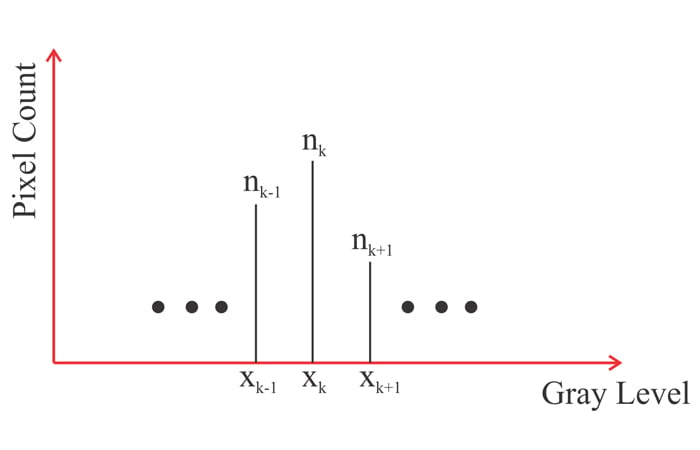
Figure 1
To equalize this histogram, we should map the pixel value xk to y given by the following equation:
\[y=f(x_k)=(L-1)\sum_{j=0}^k\frac{n_j}{N}\]
Equation 1
where L is the total number of possible gray levels (e.g. L=256 for an 8-bit image) and N is the total number of pixels in the image. The summation term \(\left ( \sum_{j=0}^k\frac{n_j}{N} \right )\) is the cumulative number of pixels whose gray value is between zero and xk.
This term is sometimes referred to as the “cumulative normalized image histogram”. Let’s look at a simple example.
A Mapping Function Example
Consider a 3-bit image with a total of 64⨉64 pixels. Assume that the histogram of this image is as shown in Figure 2.
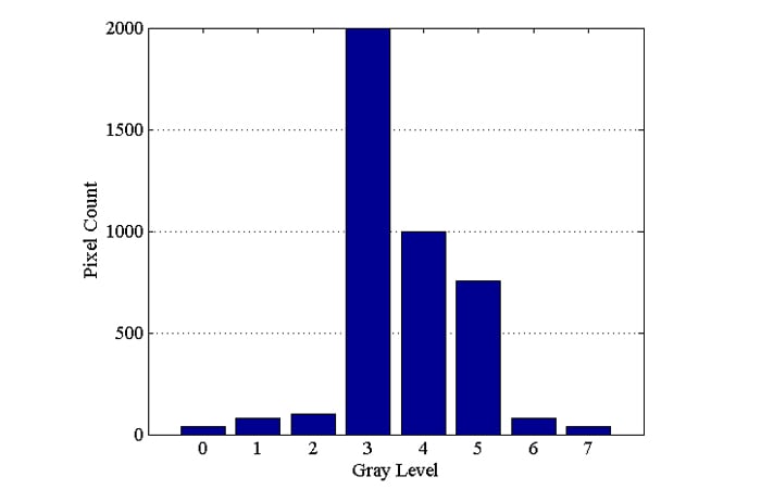
Figure 2
As you can see, there are pixel values that are much less frequent than the others. The pixel values and their number of occurrences are given in the second and third columns of Table 1, respectively.
| k | xk | nk |
y=f(xk) (from Equation 1) |
y=f(xk) (After Rounding) |
| 0 | 0 | 40 | 0.0684 | 0 |
| 1 | 1 | 80 | 0.2051 | 0 |
| 2 | 2 | 100 | 0.3760 | 0 |
| 3 | 3 | 2000 | 3.7939 | 4 |
| 4 | 4 | 1000 | 5.5029 | 6 |
| 5 | 5 | 756 | 6.7949 | 7 |
| 6 | 6 | 80 | 6.9316 | 7 |
| 7 | 7 | 40 | 7 | 7 |
Table 1
Let’s apply the mapping function of Equation 1 to this example. With a 3-bit image, there are eight different pixel values, i.e. L = 23. Substituting L = 8 and N = 64 x 64 = 4096 into Equation 1, we find the output pixel value y=f(xk) for a given input pixel value xk as given in the fourth column of the table. For example, the output of the mapping function for x4=4 can be found as \(y=f(x_4)=7\times \sum_{j=0}^4 \frac{n_j}{4096}= \frac {7}{4096} \times(40+80+100+2000+1000)=5.5029\).
Since the pixel value should be an integer, we can round this to 6 (the last column of the table). We can find the other output values for this mapping function in a similar manner.
The obtained histogram is shown in Figure 3.
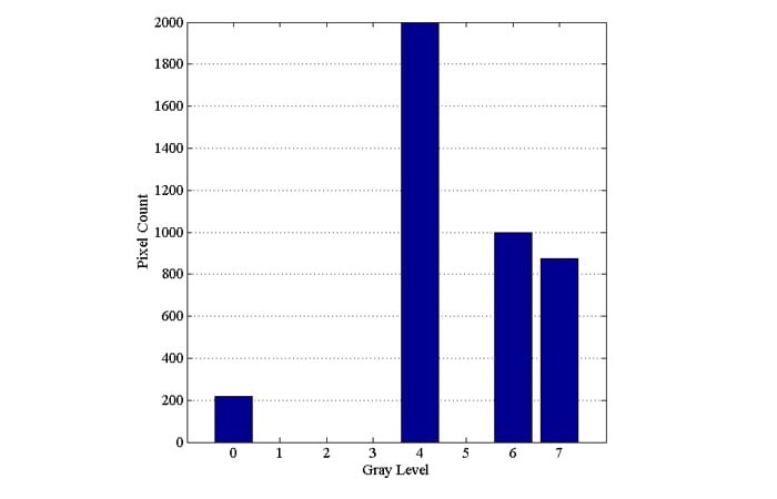
Figure 3
In this example, some of the pixel values that are less frequent, such as xk=0, 1, and 2, are mapped to a single output value (y=0). This leads to a relatively larger bin at a pixel value of zero. However, a frequent pixel value, such as xk=3, is mapped to a value (y=4) that no other input value is mapped to. Because of this, the histogram bins become relatively equalized.
This does not mean, however, that we’ll have equalized bins at all pixel values. For example, the histogram in Figure 3 shows that the bin height at a pixel value of 1 is actually reduced from 80 to zero. Therefore, when we apply the histogram equalization technique, some of the bins of the original histogram might disappear to equalize the other bins.
How Does the Cumulative Mapping Perform Histogram Equalization?
You can find the mathematical derivation of Equation 1 in textbooks (refer to Section 3.4.4 of Fundamentals of Digital Image Processing by Chris Solomon).
In this article, we’ll try to give a more intuitive explanation of how this transfer function performs histogram equalization. As with the mathematical analysis of the textbooks, we’ll first assume that the pixel value is a continuous variable and use the results to explain the discrete case.
A Continuous Case
Consider the example function shown in Figure 4. In this figure, the pixel value is a continuous variable that ranges from 0 to L-1.
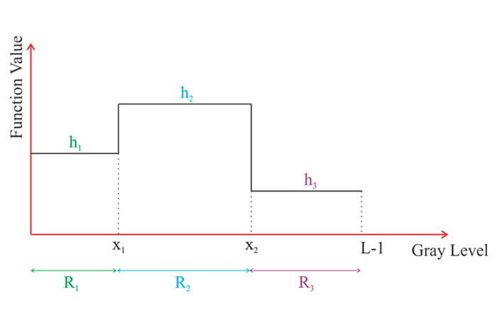
Figure 4
We need to find a mapping function that transforms the above function to the uniform function shown in Figure 5. Assuming that the total number of pixels is N, the value of the equalized function should be \(\frac {N}{L-1}\).
This is due to the fact that the integral of the function in the continuous case \(\left (\frac {N}{L-1} \times (L-1) \right )\) can be considered as the total number of pixels. In the discrete case the integral turns into a summation of the counts of the different pixel values which obviously gives the total number of pixels.
Figure 5
The original function has three different pixel value ranges denoted by R1, R2, and R3 with values h1, h2, and h3, respectively. The ranges R1, R2, and R3 are mapped to r1, r2, and r3 in Figure 5. Let’s consider the range denoted by R1.
The area of the function in this range (h1R1) indicates the number of pixels with a value between 0 and x1. All of these pixels should be mapped to the range r1 so that we obtain a flat function with a value of \(\frac {N}{L-1}\)(Figure 5). Since the total number of pixels in the range R1 is the same as the number of pixels in r1, the area h1R1 should be equal to the area of the new function in the range r1. Hence, we have:
\[h_1R_1=\frac {N}{L-1}r_1\]
This gives:
\[r_1=\frac {L-1}{N}h_1R_1\]
Equation 2
The above equation specifies the range to which the input pixel values in the range R1 are going to be mapped. A similar equation can be derived for any sub-range from 0 to x where x is less than or equal to R1. Hence, for \(x\leq R_1\), the input pixel value x should be mapped to the pixel value y given by the following equation:
\[y=\frac {L-1}{N}h_1x \;\;for \;\; x\leq R_1\]
Equation 3
This equation spreads the pixel values of the original function that reside in the range R1 over the range r1 so that the value of the output function is \(\frac{N}{L-1}\).
Similarly, the pixels in the range R2 should be mapped to the range r2 with a function value of \(\frac{N}{L-1}\)(Figure 5). Since the number of pixels is fixed, we have:
\[h_2R_2=\frac {N}{L-1}r_2\]
This gives:
\[r_2=\frac {L-1}{N}h_2R_2\]
Equation 4
Again, we can modify the above equation to obtain an equation that is valid for an arbitrary sub-range of R2. For \(x_1< x \leq x_2\) the input pixel value x should be mapped to the pixel value y given by the following equation:
\[y=r_1+ \frac{L-1}{N}h_2x\]
The first term of the above equation takes into account that the range R1 is already mapped to r1. The second term is derived from Equation 4. Substituting the value of r1 from Equation 2 gives:
\[y=\frac {L-1}{N}h_1R_1+\frac{L-1}{N}h_2x=\frac {L-1}{N}(h_1R_1+h_2x)\; \; for \;x_1< x\leq x_2\]
Equation 5
Similarly, for \(x_2 < x \leq L-1\), the input pixel value x should be mapped to the pixel value y given by the following equation:
\[y=\frac {L-1}{N}h_1R_1+\frac{L-1}{N}h_2R_2+ \frac{L-1}{N}h_3x=\frac {L-1}{N}(h_1R_1+h_2R_2+h_3x)\; \; for \;x_1< x\leq L-1\]
Equation 6
To summarize, according to Equations 3, 5, and 6, we can find the output pixel value of a given input pixel value x by calculating the integral of the original function from 0 to x and multiplying the result by \(\frac {L-1}{N}\). The above discussion is valid for the example function depicted in Figure 4.
Can we extend this result to an arbitrary function?
Note that we can use a staircase function to approximate functions of practical interest (see Figure 6). Therefore, the above result can be extended to other function types.
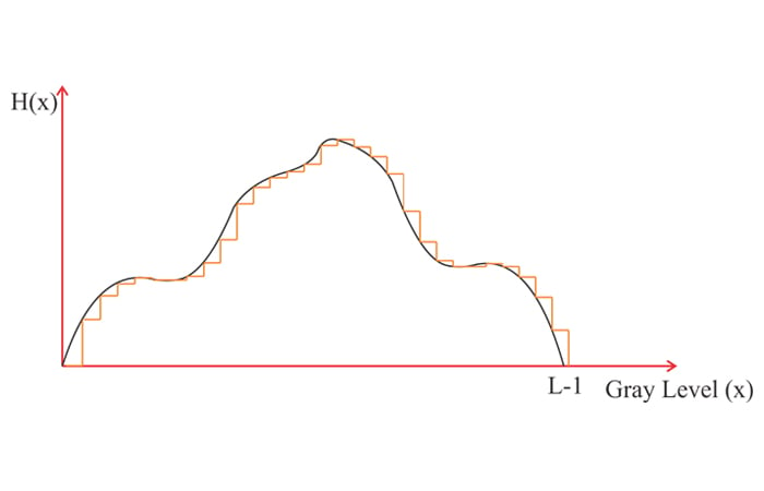
Figure 6
Hence, to find the output of the equalizing function for an input pixel value x, we integrate the original function H(x) from 0 to x and multiply the result by \(\frac {L-1}{N}\):
\[y=f(x)=\frac{(L-1)}{N}\int_0^xH(t)dt\]
Equation 7
where t is a dummy variable of integration.
Discrete Case
Intensity values in real digital images take on discrete values. In this case, the integral in Equation 7 should be replaced with a summation over the pixel counts. This gives us the equation we introduced in the first section of this article:
\[y=f(x)=\frac{(L-1)}{N}\sum_{j=0}^xn_j\]
Equation 8
It is important to note that unlike the continuous transformation, the discrete mapping cannot produce a perfectly equalized output. For example, the equalized histogram in Figure 3 had some bins of zero height. Although it cannot produce a perfectly equalized output, the discrete approximation can still lead to a flatter histogram and improve the image contrast.
Circuit Implementation
In this section, we’ll briefly look at the circuit implementation of the histogram equalization technique. We need to obtain the image histogram and use it to find the mapping function of Equation 1. A simplified block diagram for obtaining the image histogram is shown in Figure 7.
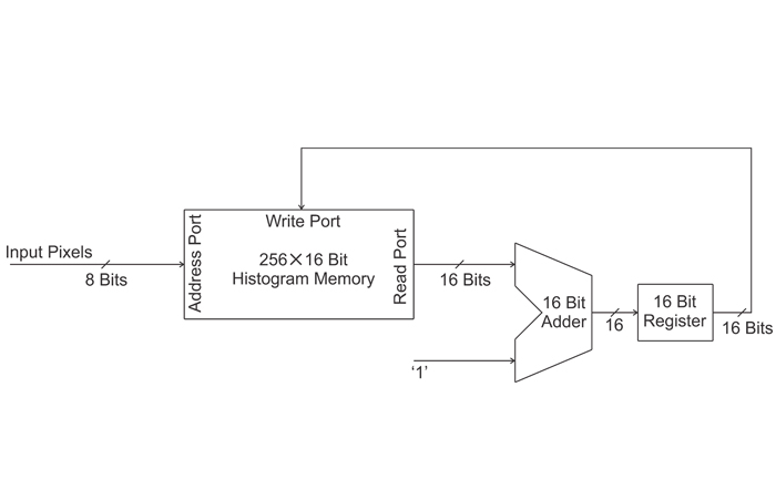
Figure 7
The memory is used to store the image histogram. In this implementation, we assume that the input is a grayscale eight-bit image of size 256 ✕ 256 pixels. An eight-bit image has 256 different pixel values. Hence, the memory should have 256 rows to store the count of the different pixel values. How many bits do we need in each row of the memory? The total number of pixels is 256 ✕ 256 = 216.
Therefore, we need a 256 ✕ 16 bit memory to be able to store the data of the worst case scenario where all of the pixels of the image are of the same value.
Initially, the memory is reset (the initial count of all of the pixel values is zero). Then, the pixel values of the input image are applied to the address port of the memory one by one. With each pixel value applied to the memory address port, the current count of that gray level appears at the read port of the memory. The current value is increased by one and the result is stored in the 16-bit register.
In the next clock cycle, the content of the register is applied to the write port of the memory to update the current count of the input pixel value. When all of the pixels are processed, the memory will contain the total count of the different pixel values (the histogram information).
To implement Equation 8, we need to calculate the sum of pixels whose gray value is in a specific range. The sum should be multiplied by L-1 and divided by N. The summation can be obtained by applying the data stored in the “Histogram Memory” to an accumulator as shown in Figure 8.
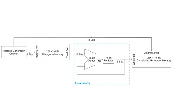
Figure 8
The “Address Generation Counter” makes the consecutive bin values of the histogram (stored in the “Histogram Memory”) appear at the input of the “Accumulator”. The current bin value is added to the sum of the previous bin values and the result is stored in the “Cumulative Histogram Memory”. The address of the “Cumulative Histogram Memory” can be obtained from the “Address Generation Counter” as well.
How can we apply the scaling factor \(\frac {L-1}{N}\) to the data of the “Cumulative Histogram Memory”?
There are several different methods. A clever technique discussed in Section 7.1.2 of the book “Design for Embedded Image Processing on FPGAs” by Donald G. Bailey modifies the structure of the accumulator to perform both the accumulation and the division in a single block. Another common technique is based on approximating the scaling factor \(\frac {L-1}{N}\). For example, with L = 256 and N = 256 ✕ 256 = 216, we have
\[\frac {(L-1)}{N}= \frac {256-1}{256 \times 256} \simeq \frac {1}{256}\]
Division by 256=28 can be simply obtained by shifting the binary data to the right by 8 bits. Hence, we can discard the lower eight bits of the data in the “Cumulative Histogram Memory” to get the output values of the equalization mapping function.
Summary
In this article, we looked at the histogram equalization technique in greater detail. We tried to develop intuition into how the mapping function of this technique flattens the image histogram. We also briefly discussed the circuit implementation of the histogram equalization method.
To see a complete list of my articles, please visit this page.
Related Content