Facebook
 Google
 GitHub
 Linkedin
Introduction to Allan Variance—Non-overlapping and Overlapping Allan Variance
Learn about non-overlapping and overlapping Allan variance and how the Allan variance curve can be used to identify different types of random errors present in a signal.
Allan variance is a statistical analysis tool for identifying various noise types that exist in a signal. Developed in the mid-1960s, the Allan variance was used to measure the frequency stability of precision oscillators. Later, this technique was applied to other areas as well. One common use case of the Allan variance is identifying the random errors that affect microelectromechanical systems (MEMS) gyroscopes.
In this article, we’ll introduce two basic versions of the Allan variance and see how the Allan variance curve can be used to identify different types of random errors present in a signal. To have a better understanding of the Allan variance technique, let’s first take a look at the signal averaging technique that is closely related to the theory behind the Allan variance.
Signal Averaging for Noise Reduction
First, let's assume that we are measuring a near-DC value affected by white Gaussian noise with a variance of:
$$\sigma^{2}_{n} = 10^{-12}$$
To reduce the noise power, we can repeat the measurement M times and average the measured values. Since the noise samples are not correlated, averaging suppresses the noise terms without affecting the value of the desired DC value. It can be shown that the noise variance of the averaged signal, $$\sigma^{2}_{n,\, avg}$$, is given by:
$$\sigma^{2}_{n,\, avg} = \frac{\sigma^{2}_{n}}{M}$$
If we plot $$\sigma^{2}_{n,\, avg}$$ against M as a log-log graph, we’ll have a line with a slope of -1. This is shown in Figure 1.
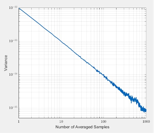
Figure 1. A graph showing variance vs number of averaged samples
Averaging more and more samples, we can reduce the noise variance from 10-12 to below 10-15. Thus, we can determine the DC input value more accurately. Although averaging can be an effective solution in certain applications, it has its own limitations: it assumes that the noise samples are not correlated with each other.
Now assume that, in addition to being affected by white Gaussian noise, our signal also slightly drifts over time. This is shown in Figure 2.
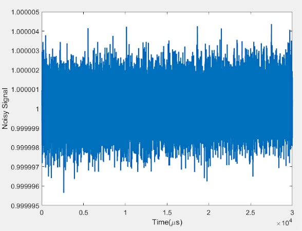
Figure 2. A graph showing how the signal drifts slightly over time.
If we apply signal averaging to the above data, we’ll obtain the brown curve below.
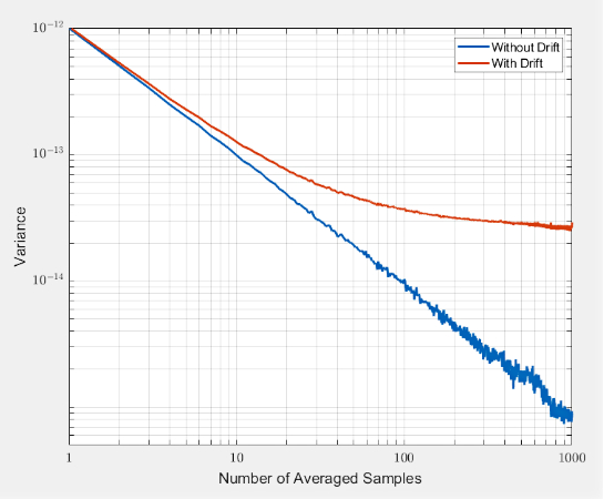
Figure 3. A graph showing the change when a signal average is undergone.
As you can see, the signal averaging technique loses its effectiveness when there is a drift in the signal. In this particular example, the variance is almost constant above about M = 200. In fact, depending on the type of the random drift affecting a given application, the variance of the averaged signal can even increase above certain values of M. Using a graph of $$\sigma^{2}_{n,\, avg}$$ against M, we can determine how many samples should be averaged to minimize the noise variance.
The Allan variance is based on a similar idea. It calculates the root mean square value of the random drift error as a function of the averaging time. Interestingly, the graph of the Allan variance doesn’t just reveal the averaging time that minimizes the noise variance, it also gives us some useful information about the different types of random processes that contribute to the drift at the circuit output.
Non-overlapping and Overlapping Allan Variance
As mentioned earlier, Allan variance was first used to measure the frequency stability of precision oscillators and has spread out to other applications. For example, the Allan variance is widely used to examine the random errors of MEMS gyroscopes. In this case, the Allan variance gives the root mean square random drift error of the gyroscope as a function of the averaging time.
Since there are several different versions of the Allan variance, we’ll take a look at the non-overlapping and fully overlapping versions of the Allen variance that are commonly used to analyze the random errors of inertial sensors. The goal will be to use the notation suitable for analyzing the output of a gyroscope.
Non-overlapping Allan Variance
To calculate the Allan variance, we need to collect a large number of samples from the gyroscope when it is motionless. To accomplish this, let's assume that we have a dataset of N samples from the gyroscope output Ω(t) at multiples of the sampling time t0. With the non-overlapping Allan variance technique, these N samples are divided into K disjoint groups of equal length where each group (or cluster) has N samples. If the sampling time is t0, the total time duration of each group is T = nt0.
Figure 4 shows the gyroscope output samples and how the clusters of the non-overlapping Allan variance are formed for n = 3.
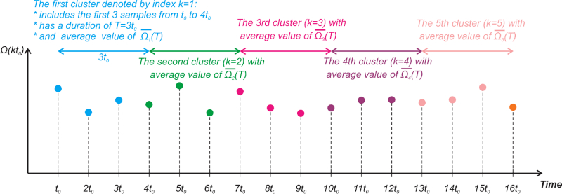
Figure 4. Example gyroscope output samples and how non-overlapping Allan variance clusters are formed.
In this example, each cluster has a time duration of 3t0. The first cluster (k = 1) includes the first 3 samples at t0, 2t0, and 3t0. The second cluster (k = 2) includes the samples at 4t0, 5t0, 6t0, and so on. To find the Allan variance, we need to calculate the average of each cluster.
The average of the kth cluster is denoted by $$\overline{\Omega}_{k}(T)$$ in Figure 4. Having the cluster averages, we can now apply the following equation to find the Allan variance:
$$\sigma^2(T) = \frac{1}{2(K-1)}\sum_{k=1}^{K-1} \Big ( \overline{\Omega}_{k+1}(T) - \overline{\Omega}_{k}(T) \Big )^2$$
Equation 1.
Note that K denotes the total number of clusters.
Overlapping Allan Variance
The overlapping Allan variance tends to perform better than a non-overlapping version for large datasets (large values of N). Similar to the non-overlapping version, the N samples from the gyroscope output Ω(t) are divided into K groups of equal length where each group (or cluster) has n samples. However, in this case, the clusters overlap each other.
Figure 5 shows how the first 6 clusters of the overlapping Allan variance are formed for n = 3.
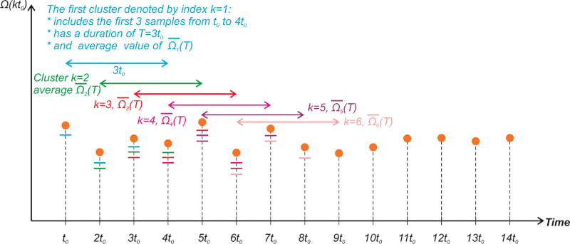
Figure 5. First six clusters of the overlapping Allan variance for n = 3.
Note that, in the overlapping version, each cluster is specified by an index k which corresponds to the first sample in the group. In the example depicted above, each cluster has a time duration of 3t0. The first cluster (k = 1) includes the first 3 samples at t0, 2t0, and 3t0. The second cluster (k = 2) includes the samples at 2t0, 3t0, 4t0, and so on. Thus, the clusters overlap each other.
The color of the short lines below the samples specifies what clusters each sample is included in. Again, to find the Allan variance, we need to calculate the average of each cluster. The average of the kth cluster is denoted by $$\overline{\Omega}_{k}(T)$$ in Figure 5.
Having the cluster averages, we can now apply the following equation to find the Allan variance:
$$\sigma^2(T) = \frac{1}{2(N-2n+1)}\sum_{k=1}^{N-2n+1} \Big ( \overline{\Omega}_{k+n}(T) - \overline{\Omega}_{k}(T) \Big )^2$$
Equation 2.
For n = 3, the first term of the above summation (k = 1) involves the cluster averages $$\overline{\Omega_{1}}_{}(T)$$ and $$\overline{\Omega_{4}}_{}(T)$$. Figure 6 shows these two clusters.
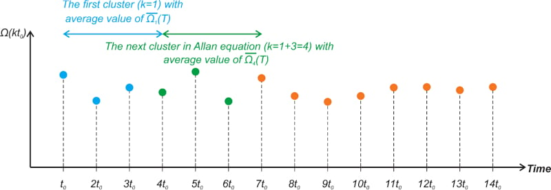
Figure 6. Example of the two overlapping Allan variance clusters.
The next term of the summation (k = 2) requires $$\overline{\Omega_{2}}_{}(T)$$ and $$\overline{\Omega_{5}}_{}(T)$$ that are shown in Figure 7.
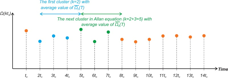
Figure 7.
Finally, taking the square root of the result obtained from either Equations 1 or 2, we obtain the value of the root Allan variance or the Allan deviation for a particular value of T.
Typical Allan Deviation Plot
The Allan deviation versus the cluster time (T) is commonly plotted in a log-log graph. Generally, the Allan variance curve is U-shaped. Figure 8 shows a typical Allan deviation curve encountered when analyzing the output of a stationary inertial sensor.
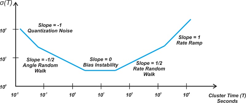
Figure 8. A general Allan deviation curve for a stationary inertial sensor.
The horizontal axis (T) can take different units in time (e.g., microseconds, seconds, minutes, or hours). The unit of the vertical axis is the angular velocity (e.g., rad/s or °/h) for gyroscopes or acceleration (given in terms of g or m/s2) in the case of accelerometers.
As you can see, depending on the value of cluster time (T), the slope of the curve can take different values. Overall, the Allan variance creates a way to identify and quantify various noise terms within the data.
There are several different random errors, such as quantization noise, angle random walk, bias instability, rate random walk, and rate ramp, that can introduce errors to the gyroscope output. Among these, quantization noise, bias instability, and rate random walk are usually the most significant effects.
To see a complete list of my articles, please visit this page.
Related Content