 Facebook
 Google
 GitHub
 Linkedin
Use Python’s Scientific Toolbox to Find the Natural Response of Thermal Systems
Use Python's scientific toolbox to determine the natural response of a real thermal system and plot the results for visualization and further analysis.
Technical Concepts Discussed: * Natural response * Differential equations * Python 3.x * C
Introduction
I'm a big fan of the Embedded.FM podcast and recently listened to Chris and Elecia White interview a guy named Matt Berggren. It was a great interview, but at one point Matt says something to the effect of, "school taught me matrices and differential equations which I haven't used since..."
I see this sort of sentiment all over the place. For the most part, unless you are in academia or very cutting edge R&D, the really technical aspects of engineering can be simplified to rules of thumb and abstracted away. A good engineer will design to 80%, not fiddle with minutiae, and iterate until the design hits the desired spec. This article is not necessarily about quickly solving an engineering problem, but peeling away the layers for a fuller understanding of the world we're trying to design in.
This article is a side note of the DIY solder reflow oven controller project I am developing in my other tutorials:
Using a simple Python script to control the oven power and log the temperature data, we can create a data file to analyze the temperature of the oven over time. Another Python script will help us determine certain properties of the oven in order to get the natural response. This article is here to fill in some gaps between the theory behind the project and the implementation using a microcontroller. It's not all about circuits, but it's still pretty cool stuff.
What You Need
Hardware
- Oven controller and TRIAC dimmer from previous tutorials
- Laptop to run test outdoors
- K-Type thermocouple and MAX31855 to measure temperature
- USB-to-Serial converter like FTDI FT232RL
Software
- Python 3
- NumPy
- Matplotlib
- SciPy
- PySerial
- Script files (attached below)
- Data logger script
- Data processing script
Warning
As a word of caution, this test may involve some pretty noxious fumes so be careful about where you run your test and which thermocouple probe you use. I purchased a $10 probe from DigiKey that was rated only to about 200 C. That rating corresponds more to the plastic insulation than to the metal filament itself – the MAX31855 can measure up to thousands of degrees given the right probe. I had to run the test outside because the oven got up to 400º C and started melting the high-temperature thermoplastic. The test ran fine but it produced some really nasty fumes and a really ugly thermocouple probe. Do your best to not breathe the fumes in. Also, be cautious of fires, burning yourself / property, or pets that may wander by not knowing any better.
The Natural Response
The natural response of a system (in our case a toaster oven) is the system's response to initial conditions with all external forces set to zero. What we would like to get out of the natural response test is an equation that estimates the behavior of the system with enough accuracy to design around.
A thermal system can be modeled as a first order differential equation, much like an RC circuit:
$$\frac{dT}{dt} + \frac{1}{\tau}T = \frac{1}{\tau}T_{a}$$
where
$$\tau = \frac{\rho c_p V}{hA_s}$$
Expanding further, $$T$$ is the temperature, $$A_s$$ is the surface area, $$\rho$$ is the density, $$c_p$$ is the specific heat, $$T_a$$ is the constant ambient temperature, and $$V$$ is the body volume.
If we turn the oven on full blast and let it reach an equilibrium temperature, when we remove power and measure the temp as it cools, it's known from Newton's Law of Cooling that the solution to this differential equation will take the form:
$$T(t)= T_0\cdot e^{-t/\tau} + T_{a}$$
$$T_0$$ is the temperature above ambient, $$\tau$$ is the thermal time constant, and $$T_a$$ is again the ambient temperature.
$$\tau$$, being the thermal time constant, according to this U.S. Sensor Whitepaper also corresponds to:
"...the time required for [the oven] to change 63.2% of the total difference between its initial and final body temperature when subjected to a step function change in temperature, under zero power conditions".
This is a quantity that can be measured from the collected data. Now that we have an equation, we can use Python to automate the collection of temperature data and then smack it around using the SciPy optimization toolbox to get the values that fill up the equation.
The Software
If you're new to Python or scientific computing, I'd recommend giving Anaconda from Continuum a shot. I don't have any association with them (and neither does AAC), but it's a pretty useful software package. It's a cross-platform Python distribution that provides support for all the scientific libraries, virtual environments, package management, IDE, and some other nice-to-haves. I'm using the Python 3.5 version.
There are three "moving parts" to this article:
- A working oven controller that can interpret UART commands
- This has been covered in previous tutorials and only relevant source files to the natural response test will be provided.
- A script that can control the oven power though the UART and measure the temperature for data logging
- This is a fast and dirty script that just sets the oven to full power and logs the temp until you tell it to stop
- A script to post-process the data and fit a curve to the sampled temperature values
- This digs into the Python scientific toolbox for plotting and such
ATMega328P UART Command Interface
The oven's microcontroller code can be seen below. It's a modified version of Colin N. Brosseau's code which parses UART commands and runs predefined functions based on the input.
/*
Copyright (c) 2013, Colin-N. Brosseau
All rights reserved.
Redistribution and use in source and binary forms, with or without
modification, are permitted provided that the following conditions are met:
1. Redistributions of source code must retain the above copyright notice, this
   list of conditions and the following disclaimer.
2. Redistributions in binary form must reproduce the above copyright notice,
   this list of conditions and the following disclaimer in the documentation
   and/or other materials provided with the distribution.
THIS SOFTWARE IS PROVIDED BY THE COPYRIGHT HOLDERS AND CONTRIBUTORS "AS IS" AND
ANY EXPRESS OR IMPLIED WARRANTIES, INCLUDING, BUT NOT LIMITED TO, THE IMPLIED
WARRANTIES OF MERCHANTABILITY AND FITNESS FOR A PARTICULAR PURPOSE ARE
DISCLAIMED. IN NO EVENT SHALL THE COPYRIGHT OWNER OR CONTRIBUTORS BE LIABLE FOR
ANY DIRECT, INDIRECT, INCIDENTAL, SPECIAL, EXEMPLARY, OR CONSEQUENTIAL DAMAGES
(INCLUDING, BUT NOT LIMITED TO, PROCUREMENT OF SUBSTITUTE GOODS OR SERVICES;
LOSS OF USE, DATA, OR PROFITS; OR BUSINESS INTERRUPTION) HOWEVER CAUSED AND
ON ANY THEORY OF LIABILITY, WHETHER IN CONTRACT, STRICT LIABILITY, OR TORT
(INCLUDING NEGLIGENCE OR OTHERWISE) ARISING IN ANY WAY OUT OF THE USE OF THIS
SOFTWARE, EVEN IF ADVISED OF THE POSSIBILITY OF SUCH DAMAGE. */

#include "globals.h"

unsigned char _data_count = 0;
int _variable_A = 23; //user modifiable variable
int _variable_goto = 12; //user modifiable variable
unsigned char _data_in[8] = {0};
char _command_in[8] = {0};


int cmd_parseAssignment (char input[16])
{
    char *pch;
    char cmdValue[16];

    // Find the position the equals sign is
    // in the string, keep a pointer to it
    pch = strchr(input, '=');

    // Copy everything after that point into
    // the buffer variable
    strcpy(cmdValue, pch+1);

    // Now turn this value into an integer and
    // return it to the caller.
    return atoi(cmdValue);
}

void cmd_copyCommand (void)
{
    // Copy the contents of data_in into command_in
    memcpy(_command_in, _data_in, 8);

    // Now clear _data_in, the UART can reuse it now
    memset(_data_in, 0, 8);
}

void cmd_processCommand(max31855 *tempSense)
{
    if(strcasestr(_command_in, "g") != NULL)
    {
        if(strcasestr(_command_in, "t") != NULL)
        {
            if(strcasestr(_command_in, "e") != NULL)
                cmd_printValue("TC Temp", tempSense->extTemp, ID_OFF);

            if(strcasestr(_command_in, "i") != NULL)
                cmd_printValue("RJ Temp", tempSense->intTemp, ID_OFF);
        }

        if(strcasestr(_command_in, "s") != NULL)
        {
            uart0_puts(max31855_statusString(tempSense->status));
            uart0_puts(RETURN_NEWLINE);
        }
    }

    if(strcasestr(_command_in, "s") != NULL)
    {
        // If set is true, assume a '=' in cmd and send to cmd_parseAssignment
        int tmpcmd = cmd_parseAssignment(_command_in);

        // if(strcasestr(_command_in, "f") != NULL)
        // {
        //
        //     if (tmpcmd > 0)
        //         oven_fade(tmpcmd);
        // }

        if(strcasestr(_command_in, "p") != NULL)
        {
            if(tmpcmd >= 0 && tmpcmd <= 100)
                oven_setDutyCycle(tmpcmd);
        }
    }
}

void cmd_printValue (char *id, int value, uint8_t printID)
{
    char buffer[8];
    itoa(value, buffer, 10);

    if(printID)
    {
        uart0_puts(id);
        uart0_puts_P(" = ");
    }

    uart0_puts(buffer);
    uart0_puts_P(RETURN_NEWLINE);
}

void cmd_uartOK(void)
{
  uart0_puts_P("OK");
  uart0_puts_P(RETURN_NEWLINE);
}

void cmd_processUART(max31855 *tempSense)
{
    /* Get received character from ringbuffer
    * uart0_getc() returns in the lower byte the received character and
    * in the higher byte (bitmask) the last receive error
    * UART_NO_DATA is returned when no data is available.   */
    unsigned int c = uart0_getc();

    if ( !(c & UART_NO_DATA) )
    {
        // new data available from UART check for Frame or Overrun error
        if ( c & UART_FRAME_ERROR ) {
            /* Framing Error detected, i.e no stop bit detected */
            uart0_puts_P("UART Frame Error: ");
        }
        if ( c & UART_OVERRUN_ERROR ) {
            /* Overrun, a character already present in the UART UDR register was
            * not read by the interrupt handler before the next character arrived,
            * one or more received characters have been dropped */
            uart0_puts_P("UART Overrun Error: ");
        }
        if ( c & UART_BUFFER_OVERFLOW ) {
            /* We are not reading the receive buffer fast enough,
            * one or more received character have been dropped  */
            uart0_puts_P("Buffer overflow error: ");
        }

        // Add char to input buffer
        _data_in[_data_count] = c;

        // Return is signal for end of command input
        if (_data_in[_data_count] == CHAR_RETURN)
        {
            // Reset to 0, ready to go again
            _data_count = 0;
            //uart0_puts(RETURN_NEWLINE);

            cmd_copyCommand();
            cmd_processCommand(tempSense);
            //cmd_uartOK();
        }
        else _data_count++;

        //uart0_putc( (unsigned char)c );
    }
}
This code reads data from the UART buffer and parses out commands and value assignments. The cmd_processCommand(*max31855 tempSense) section shows which commands are set up. A command with a 'g' is a 'get info' statement and doesn't require an argument; a command with an 's' is a 'set value' command and requires that you have a '=' character and an integer value following it. For example, to set the oven power to 75%, you would send: sp=75.
Python Oven Interface and Data Logger
The next step is to write a Python script that can read and write to the UART using the PySerial library. The automated script assumes /dev/ttyUSB0 is the serial port to interact with and can be modified for your particular device.
import time
import sys
import serial
import csv
from datetime import datetime

def countdown(t):
    while t:
        mins, secs = divmod(t, 60)
        timeformat = '{:02d}:{:02d}'.format(mins, secs)
        print(timeformat, end='\r')
        time.sleep(1)
        t -= 1

# Set up the port
ser = serial.Serial('/dev/ttyUSB0', 9600, timeout = 1)

oven_on = ("sp=100\r\n").encode('ascii')
oven_off = ("sp=0\r\n").encode('ascii')
get_tctemp = ("gte\r\n").encode('ascii')

ser.write(oven_off)

print('Measure step response of toaster')
print('Please ensure toaster is at ambient temp.')
print('Press ENTER to begin and <CTRL>+C to end.')
input('>>> ')

csv_file = open('stepresponse.csv', 'w', newline='')
writer = csv.writer(csv_file)

# Read some temps
print('Starting in')
countdown(5)

# Write some stuff to the oven
ser.write(oven_on)

try:
    while(True):
        ser.write(get_tctemp)
        tc_temp = (ser.readline()).decode('ascii')
        tc_temp = tc_temp.rstrip()

        print(tc_temp)
        writer.writerow([datetime.now(), tc_temp])

        time.sleep(0.01)

except KeyboardInterrupt:
    print("Interrupted. Closing CSV.")
    csv_file.close()
    ser.write(oven_off)
This script opens the /dev/ttyUSB0 serial port, waits for the user to hit ENTER, counts down, and then turns the oven on full. There's a while loop in place that continuously reads the temperature, gives it a timestamp, and writes it all to a CSV file. When you decide to finish the test, hit CTRL+C to cancel and close the CSV file.
Python Curve Fitting
The following is the meat and potatoes of the tutorial, and is the most project agnostic. It uses NumPy vectors to work with the numerical data, Matplotlib's PyPlot to display the data, and the SciPy optimization toolbox to fit a curve to the sampled data we got from the test.
import csv
import sys
import numpy as np
import matplotlib.pyplot as plt
from scipy.optimize import curve_fit
from datetime import datetime, timedelta

# Define the exponential function we want to fit a curve to
def exponential(x, a, b, c):
    return a * np.exp(-b * x) + c

# Open CSV file in read+binary mode
#f = open(sys.argv[1], newline='')
f = open('natural-response.csv', newline='')

# Lists for CSV Datas
timestamp = []
tempdata = []

# Read the CSV file and convert the data back into more useful types
try:
    reader = csv.reader(f)
    for row in reader:
        timestamp.append(datetime.strptime(row[0], '%Y-%m-%d %H:%M:%S.%f'))
        tempdata.append(int(row[1]))
finally:
    f.close()

# Determine from timestamps an array t with elements
# equal to the time after beginning test
t = []
for entry in timestamp:
    delta = entry - timestamp[0]
    t.append(delta.seconds + delta.microseconds / 1000000)

# Numbered list from 0 to however big the array is. This is not used but I
# figured it out while making this script and I think it's a cool expression
# x = [i for i in range(len(tempdata))]

# Determine thermal time constant. During cooldown, find time to go from
# max temp to 63% of max temp.
tc = t[next(i[0] for i in enumerate(tempdata) if i[1] < 236)]

# Numpy stop being dumb and just let me use t as an argument!
popt, pcov = curve_fit(exponential, np.array(t), tempdata, p0 = (400, 1/tc, 27))
guess = exponential(np.array(t), *popt)
print('System parameters\n-----------------')
print('Estimated thermal time constant: {0} seconds'.format(tc))
print('Optimized thermal time constant: {0} seconds'.format(1/popt[1]))

print('Optimized values:')
print('y(0) = {0}, 1/TC = {1}, c = {2}'.format(*popt))

# Put everything onto a plot
plt.figure()
plt.plot(t, tempdata, 'b-', linewidth = 2, label="Original Sampled Data")
plt.plot(t, guess, 'r-', label="Fitted Curve")
plt.legend()
plt.show()
The actual curve fitting is done with popt, pcov = curve_fit(exponential, np.array(t), tempdata, p0 = (400, 1/tc, 27)). It requires a best guess of initial values and because we know the system is a first order exponential, has an initial value of 400º C, ambient temperature around 30º C, and has a measurable time constant, we can feed all that back into the function to get our result.
The script prints out the fitted equation and then plots the data as well as the estimated line:
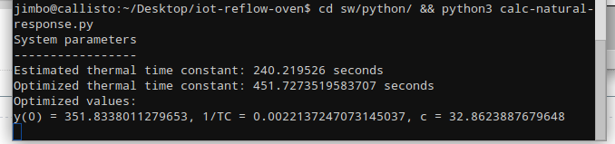
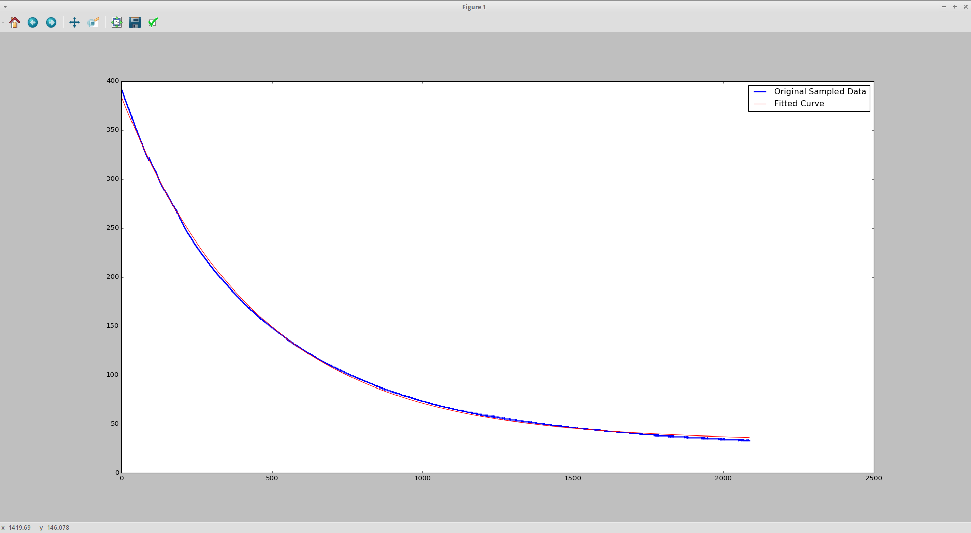
This gives us a final equation of
$$T(t)= 351.8\cdot e^{-t/451.7} + 32.9$$
If you look at the code, you can see that my guess for the thermal time constant and initial temp above ambient weren't correct, but it didn't matter to the curve fitting algorithm. It really just needs a ballpark estimate and then it will iterate with numerical methods to find the best solution.
Conclusion
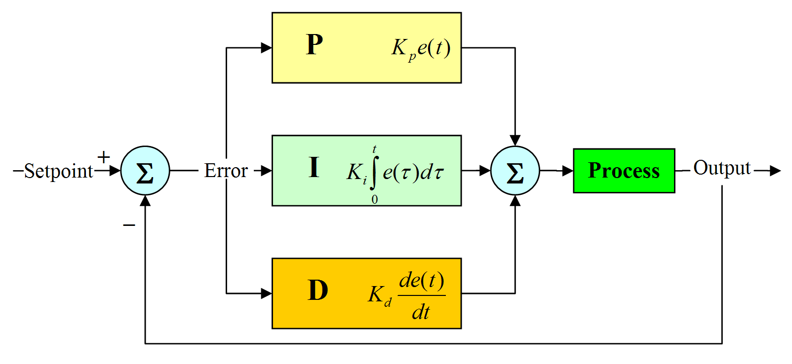
Now that we have a practical model of our oven, we can use this as a plant/process model for building the temperature control system. The next step is to take the Laplace transform of our oven equation, and build a transfer function for which we can add feedback and various controller blocks. For example, the ubiquitous PID controller (which our oven project will use) can be represented in a feedback loop with our model like so:
No model created can ever capture perfectly all the tiny details of physics that could have an effect on what we're designing. Inescapable facts of life like measurement noise, quantization error, changes in ambient temperature, the thermal properties of whatever we put inside the oven, etc. will all make the real system behave differently than the prediction. Still, it is possible to create a fast and robust controller by starting with as accurate a model as possible and applying good control system design principles to achieve the desired result. I'll leave you with one final bit of wisdom from George E. P. Box to consider:
"Essentially, all models are wrong, but some are useful."
Until next time... happy hacking.
All code files for the project can be found here:
Related Content


Thanks for the detailed write-up. I think your time constant estimate was so far off because you swapped from a step response (increasing) to a decay (decreasing) experiment. Therefore your estimate should be based on a 37% threshold, not 63%.