 Facebook
 Google
 GitHub
 Linkedin
Negative Feedback, Part 2: Improving Gain Sensitivity and Bandwidth
Having introduced the general negative feedback structure, we will now demonstrate that negative feedback has a beneficial effect on two important characteristics of amplifier circuits.
Having introduced the general negative feedback structure, we will now demonstrate that negative feedback has a beneficial effect on two important characteristics of amplifier circuits.
Previous Article in This Series
Supporting Information
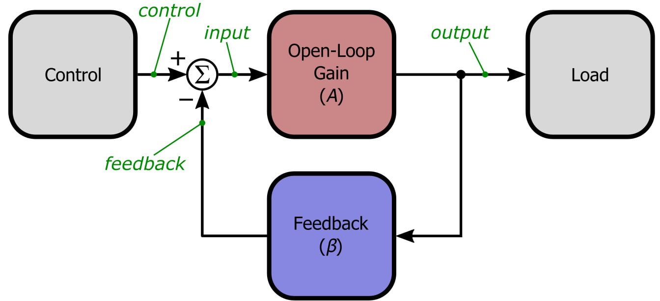
Just so you don't have to switch pages every time you want to ponder the general feedback structure, here is the diagram presented in the previous article:
The Fundamental Trade-Off
In the previous article we saw that incorporating negative feedback changed the overall gain of an amplifier circuit from A (i.e., the open-loop gain of the original amplifier) to approximately 1/β, where β is the feedback factor, that is, the percentage of the output that is fed back and subtracted from the control (or reference) signal. But now we face an important question: What’s wrong with A? Why not just design the open-loop amplifier to have the gain we want and forget about negative feedback?
Well, theoretically that should work, but in reality it is much easier to achieve precise, consistent gain with a simple feedback network than with an amplifier. Take a look at these numbers for the LT6003 op-amp from Linear Technology:
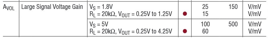
Here we have the open-loop gain specs for a modern general purpose op-amp from a leading analog IC manufacturer. How would you feel about an 80% reduction in the gain of your mission-critical amplifier circuit? Notice, though, that these gains are quite high—ranging from a worst case of 15,000 V/V to a nominal value of 500,000 V/V at Vsupply = 5 V. What we could rightly conclude, then, is the following: it is difficult to design a general purpose amplifier with precise, consistent gain, and it is easy to design a general purpose amplifier with very high gain. As you have probably realized by now, negative feedback is the perfect solution to this quandary: the simple passive components that constitute the feedback network provide precision and consistency, and the very high open-loop gain of the amplifier makes the closed-loop gain less sensitive to the sort of extreme variation that you see in the specs given above. This exemplifies the fundamental trade-off of a negative feedback amplifier—we reduce the overall gain in order to improve the circuit in other ways. So let’s take a closer look at our first negative feedback benefit: gain desensitization.
It’s Good to Become Less Sensitive
We have already discussed feedback’s ability to make an amplifier dependent on β instead of A, so we’ll be brief here. By “gain desensitization” we mean that the closed-loop gain of the amplifier-plus-feedback circuit is much less sensitive to variations in the amplifier’s open-loop gain. The point we have not yet explicitly made is that greater desensitization is achieved when the open-loop gain is higher and the closed-loop gain is lower. Recall the formula for closed-loop gain:
\[G_{CL}=\frac{A}{1+A\beta}\]
We can intuitively observe that any change in A is divided by (1 + Aβ) before it affects the closed-loop gain. With a little calculus, you can indeed confirm that the ratio GCL,old/GCL,new is reduced by the factor (1 + Aβ) relative to Aold/Anew. Thus, when A is very large—as it is in standard op-amps—and β is restricted to typical values (say, not less than 0.01, corresponding to a gain of 100), the quantity (1 + Aβ) is large enough to ensure that the closed-loop gain is minimally affected by variations in A. For example, imagine that the open-loop gain of an op-amp increases by 10% as a result of changes in ambient temperature, with a starting open-loop gain of 100,000. The feedback network is designed for a gain of 10.
\[G_{CL,old}=\frac{100,000}{1+\left(100,000\times0.1\right)}=9.99900,\ \ \ \ \ \ \ \ \ G_{CL,new}=\frac{110,000}{1+\left(110,000\times0.1\right)}=9.99909\]
It is safe to say that most systems would not be seriously impaired by a 0.00009 V/V increase in amplifier gain.
Widen Your Band
As mentioned in the previous article, real-life amplifiers don’t have a single gain value that applies to signals of any frequency. Most op-amps are internally compensated to make them more stable, resulting in an open-loop gain that decreases at 20 dB/decade starting at very low frequencies. And even in devices that are specifically designed and optimized for high-frequency operation, parasitic inductances and capacitances will eventually cause the gain to roll off. But don’t let these bandwidth limitations discourage you—negative feedback can help.
Now that we are considering the amplifier’s frequency response, we should modify the closed-loop gain equation as follows, where GCL,LF and ALF denote the closed-loop and open-loop gain at frequencies much lower than the open-loop cutoff frequency.
\[G_{CL,LF}=\frac{A_{LF}}{1+A_{LF}\beta}\]
Nothing too surprising here. The interesting thing is what happens to the frequency response; if you analyze the closed-loop gain as a function of frequency, you will find that the closed-loop cutoff frequency (fC,CL) is related to the open-loop cutoff frequency (fC,OL) as follows:
\[f_{C,CL}=f_{C,OL}\left(1+A_{LF}\beta\right)\]
Thus, we actually get significantly more usable bandwidth in the amplifier-plus-feedback circuit. Note also that, as with gain desensitization, higher open-loop gain leads to greater improvement in bandwidth.
Perhaps you have noticed something interesting here: the bandwidth is increased by the factor (1 + ALFβ) and the low-frequency gain is reduced by the factor (1 + ALFβ). This leads to the rather elegant relationship whereby decreasing the gain of the amplifier by a certain factor causes the bandwidth to increase by the same factor. This is best clarified with some frequency response plots. Here is the open-loop gain of the LT1638, a general purpose op-amp from Linear Tech.
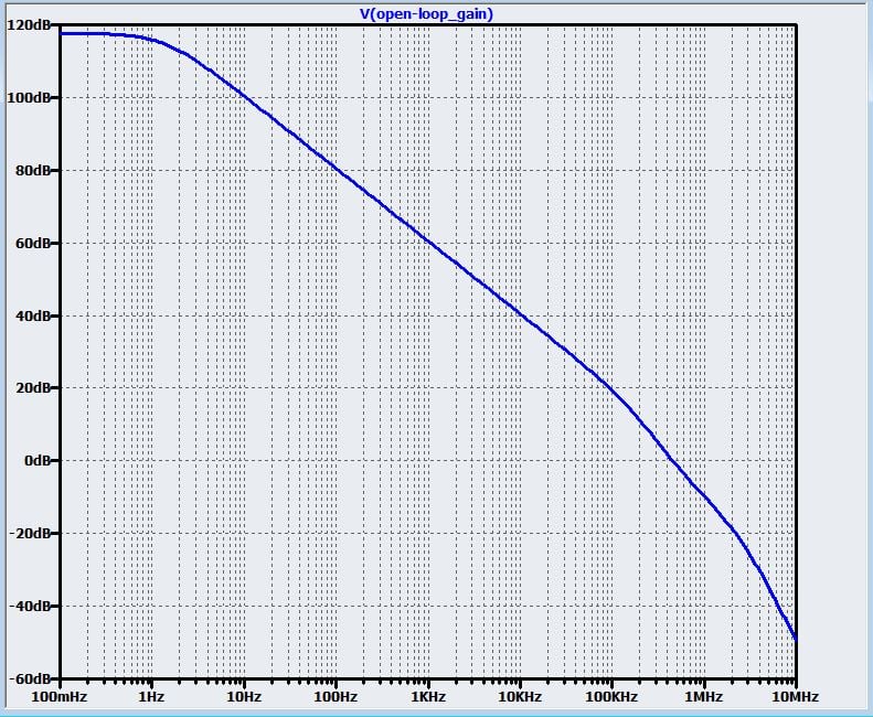
As expected, we have a 20 dB/decade roll-off beginning at very low frequencies. Now let’s add feedback with β = 0.1 (corresponding to a gain of 10).
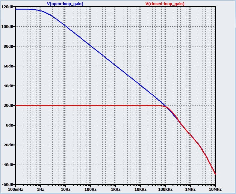
In this circuit, (1 + ALFβ) ≈ (1 + 708,000×0.1) = 70,801 = 97 dB. We can readily confirm from the plot that the gain is indeed reduced by 97 dB. In the next plot the cursors are located near the two cutoff frequencies.
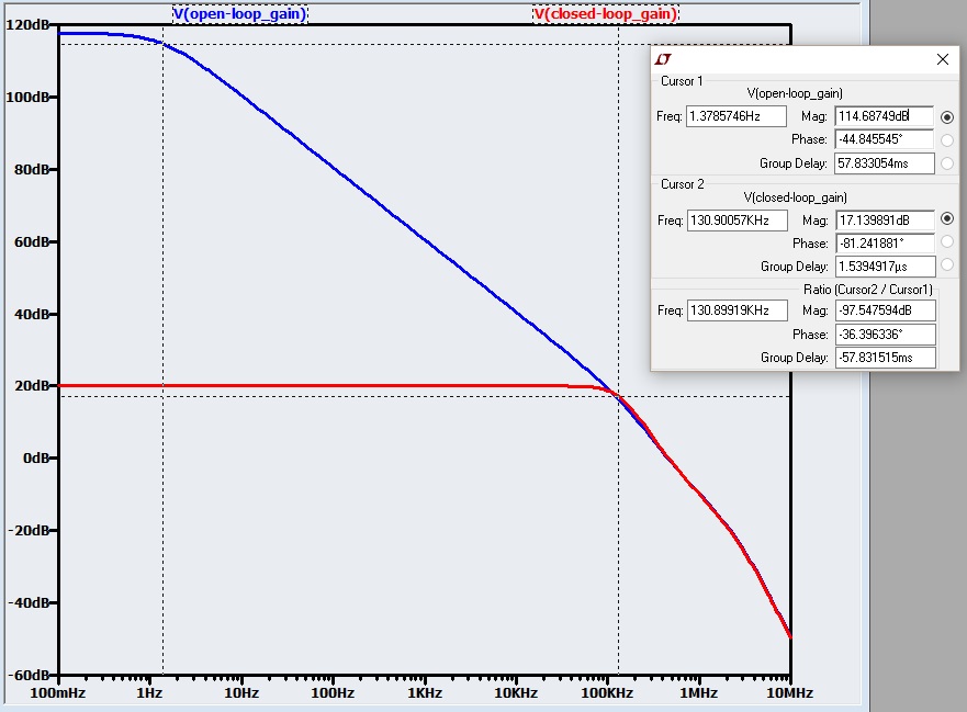
The bandwidth is extended by a factor of 130,900/1.38 = 94,855, which is consistent with the expected ratio but not exactly what we would predict. The results here are less precise than with gain because the expected mathematical relationships assume an ideal one-pole frequency response, whereas a one-pole response is only an approximation of an op-amp’s actual open-loop gain vs. frequency characteristics.
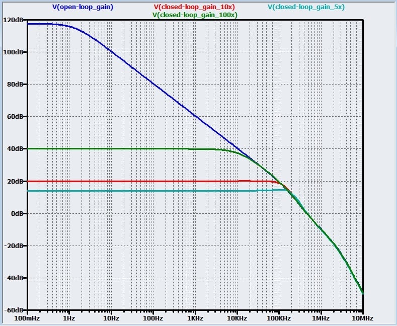
The next plot, which includes curves for two additional feedback networks, helps to illustrate the inverse relationship between closed-loop gain and closed-loop bandwidth: as gain goes up, bandwidth goes down.
Gain-Bandwidth Product Equals . . . Product of Gain and Bandwidth
The foregoing discussion should help you to understand why op-amp manufacturers can concisely convey the high-frequency performance of their devices using one simple specification, namely, the gain-bandwidth product, abbreviated GBP. (Note that GBP is applicable to voltage-feedback op-amps, not current-feedback op-amps.)
\[f_{GBP}=f_{C,OL}\times A_{LF}=f_{C,CL}\times G_{CL,LF}\]
The above formula expresses both how the GBP is determined and how it is used. To find the GBP, multiply the open-loop gain by the open-loop cutoff frequency (in practice, though, you don’t calculate the GBP because it is given to you in the op-amp datasheet). To use the GBP in the design process, you plug in your desired gain or bandwidth to determine the corresponding maximum bandwidth or gain that this particular amplifier can achieve. (In an actual design you would always factor in some margin—e.g., if you need a gain of 10 from 0 Hz to 1 MHz, look for an op-amp with a GBP of at least 30 MHz, preferably 50 MHz.)
One last observation: The above formula implies that the GBP is the same as the op-amp’s unity-gain frequency, since plugging in 1 for GCL,LF means that fGBP = fC,CL. However, keep in mind that the unity-gain frequency of an amplifier is not always the same as the GBP: the GBP is determined by the low-frequency open-loop gain and the open-loop cutoff frequency, whereas the unity-gain frequency is the frequency at which the open-loop gain equals 1. If the amplifier has a second (non-dominant) pole that increases the roll-off slope before the open-loop gain reaches 1, the unity-gain frequency will be lower than the GBP.
Conclusion
We are now well aware that negative feedback can improve two critical amplifier characteristics—bandwidth and sensitivity to open-loop gain—while costing us little more than a simple feedback network and some gain that we didn’t need anyways. In the next article we will consider negative feedback’s beneficial effect on some other less-prominent but nonetheless important properties of amplifier circuits.
Next Article in Series: Negative Feedback Part 3: Improving Noise, Linearity, and Impedance


Great explanation.Can you explain the Linear Tech example more in detail.Thanks
Great job!
Suggestion: for completeness, it would be good to mention how did you simulate open-loop gain of the LT1638.