Negative Feedback, Part 9: Breaking the Loop

A simple “break-the-feedback-loop” simulation technique makes for convenient stability analysis, especially with complex circuits.

Previous Articles in This Series

• Negative Feedback, Part 1: General Structure and Essential Concepts
• Negative Feedback, Part 2: Improving Gain Sensitivity and Bandwidth
• 316207Negative Feedback, Part 3: Improving Noise, Linearity, and Impedance324
• Negative Feedback, Part 4: Introduction to Stability325
• Negative Feedback, Part 5: Gain Margin and Phase Margin326
• Negative Feedback, Part 6: New and Improved Stability Analysis
• Negative Feedback, Part 7: Frequency-Dependent Feedback
• 327Negative Feedback, Part 8: Analyzing Transimpedance Amplifier Stability500471

Supporting Information

• Introduction to Operational Amplifiers
• Operational Amplifiers: Negative Feedback329
• AC Phase
• Introduction to SPICE504475

Elusive Loop Gain

You may have realized by now that there is something mildly troublesome about stability analysis—somehow it is just not as straightforward as it should be. After some reflection, you probably identified the source of this inherent inconvenience: the loop gain. As we now are well aware, stability is fundamentally dependent on the frequency response of the loop gain Aβ; the problem is, loop gain is not a measurable or even intuitive quantity in actual circuits. The open-loop gain A is an intuitive and measurable quantity: apply a test signal to the amplifier itself, without any feedback, and measure the output. Likewise, the closed-loop gain is intuitive and measurable: assemble (or simulate) the circuit and measure the output relative to the input. Loop gain, in contrast, is “hidden” inside the externally observable voltages and currents.

So what happens when you need to investigate the stability of a complex feedback amplifier? Or what if you simply don’t like the somewhat “manual” approach adopted in previous articles, where we treated the feedback network as a partially separate circuit and combined the feedback voltage with the open-loop response to generate the necessary stability-analysis plots? Well, it turns out that there is a well-defined method for extracting the loop gain from an existing circuit.

The Broken Loop

The following diagram shows the general feedback structure introduced in the first article, but with one important modification: the feedback network has been separated from the output, and a test signal is injected at the point of separation.

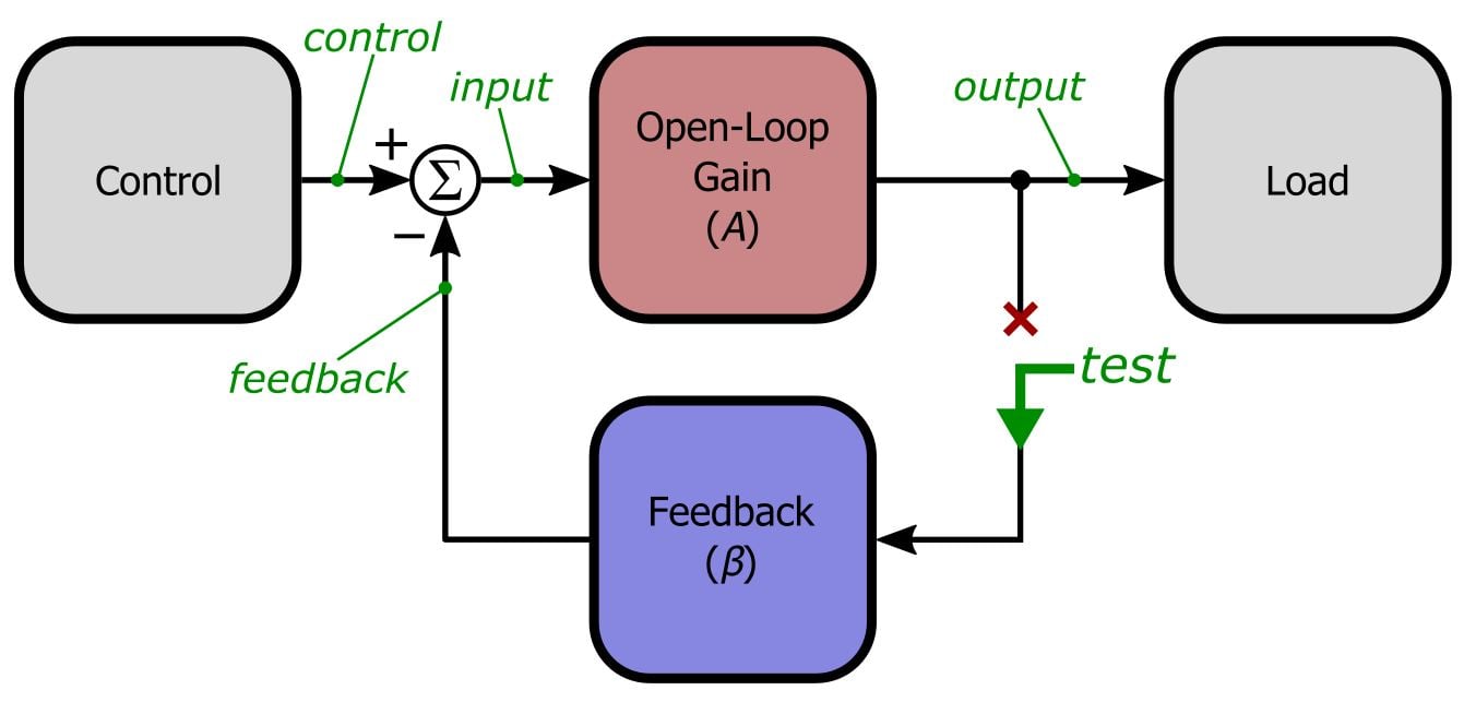
If you remove (i.e., set to zero) the input to the overall system (here denoted by control) and then examine the signal flow through this new structure, you will see that the following relationships are now in play:

\[input=0-\beta test\ \ \Rightarrow\ \ output=-A\beta test\ \ \Rightarrow\ \ \frac{output}{test}=-A\beta\]

In our simulations we will always use a test voltage of 1 V, so we can simplify this as follows:

\[A\beta=-output\]

Thus, when we break the feedback loop and inject a 1 V test signal into the feedback network, the output of the amplifier, multiplied by negative 1, is the loop gain. Theoretically this approach could be used to investigate loop gain using mathematical analysis, simulations, or even a real circuit along with a variable frequency AC test signal. But practical difficulties arise with the mathematical and measurement approaches, primarily because it is theoretically necessary to terminate the broken loop with an impedance equivalent to the impedance that existed before the loop was broken. So without further ado we will move on to a simulation-based manifestation of this method—the fact is, in this context simulations are usually (if not always) the least tedious and most informative approach.

Yet Another Pole to Worry About

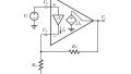
We know from previous articles that poles can cause trouble for those who want stable amplifiers. Internally compensated op-amps have a single pole that dominates the frequency response, thus ensuring stability in most situations. But a pole in the feedback network, created by capacitance in parallel with a feedback resistor, can provide enough additional phase shift to degrade stability. Unfortunately, there is another place where (often unintentional) capacitance can stir up oscillations—namely, at the op-amp’s output node:

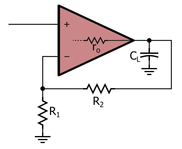
As you can see, any load capacitance connected directly to the output combines with the op-amp’s (small but nonzero) output impedance to form an RC circuit—in other words, a single-pole low-pass filter that contributes an additional 90° of phase shift to the loop gain’s frequency response.

Of course, there is always at least some small amount of parasitic capacitance. How much load capacitance does it take to actually destabilize a circuit? The simplest way to determine this is to check the datasheet, which should indicate how much load capacitance a particular op-amp can safely drive. The datasheet might provide a numerical specification for this, or it might give you a plot showing overshoot percentage for different values of load capacitance. Here is an example of the latter, taken from the datasheet for the AD8505 op-amp manufactured by Analog Devices:

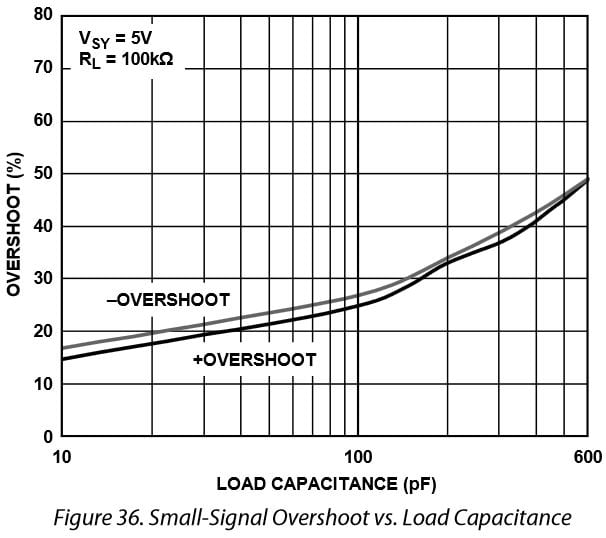
Overshoot greater than about 20% indicates inadequate phase margin, so with the AD8505, load capacitance as low as 30 pF is enough to cause concern.

The Technique

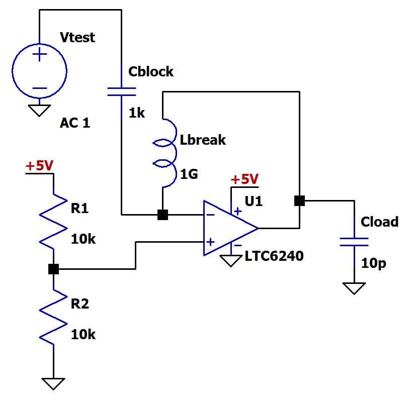
Let’s say that we are using an op-amp to provide a voltage reference equal to V_DD/2, as follows:

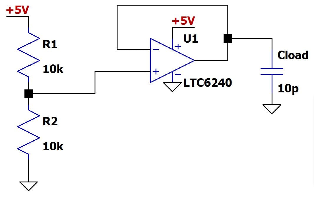
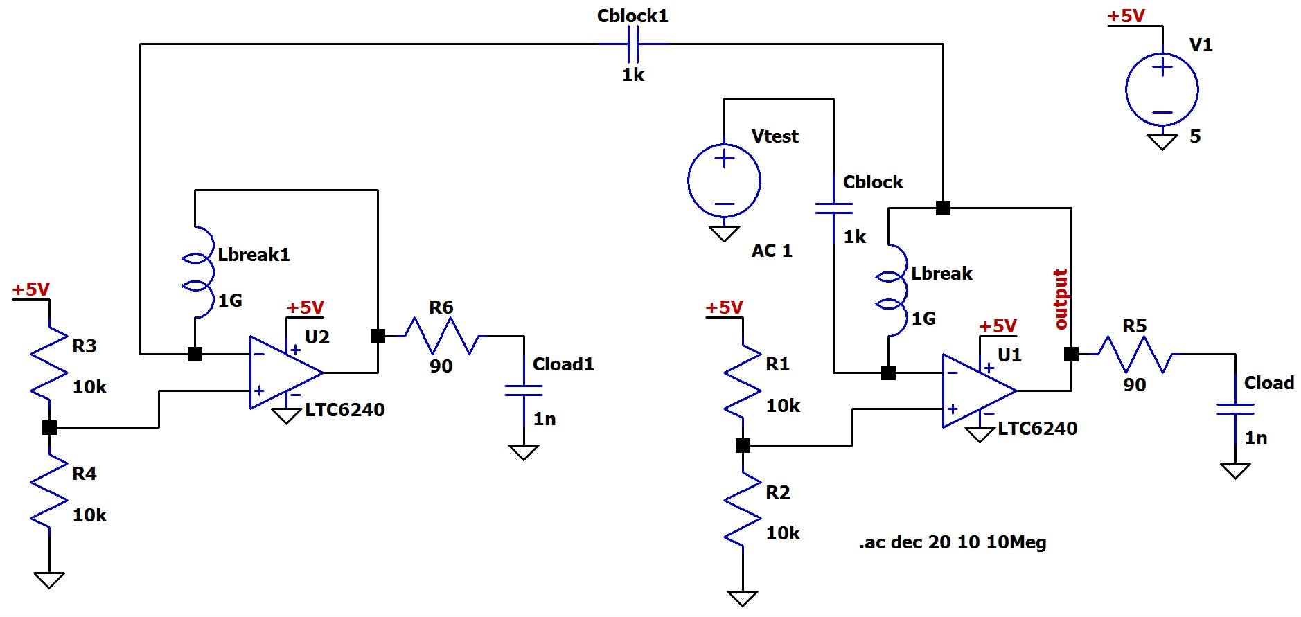
The current value of C_load represents parasitic capacitance. Let’s check this circuit’s stability using a break-the-loop approach. We need to ensure that the simulator can establish proper DC bias conditions, so we break the loop not with an open circuit but with a very large (1 GH) inductor. This unrealistically large inductor, with a theoretical impedance of zero at DC, allows for proper DC biasing while effectively blocking all AC signals of interest. Similarly, we inject the 1 V AC test signal through a large capacitor, which blocks DC but presents essentially no impedance to AC signals.

We’re not done quite yet . . . we still need to terminate the feedback network with the impedance that existed before we broke the loop. There is a simple, though by no means elegant, way to accomplish this: copy and paste the entire circuit and use this duplicate as a dummy load; because it is the same circuit, it will provide the proper termination impedance.

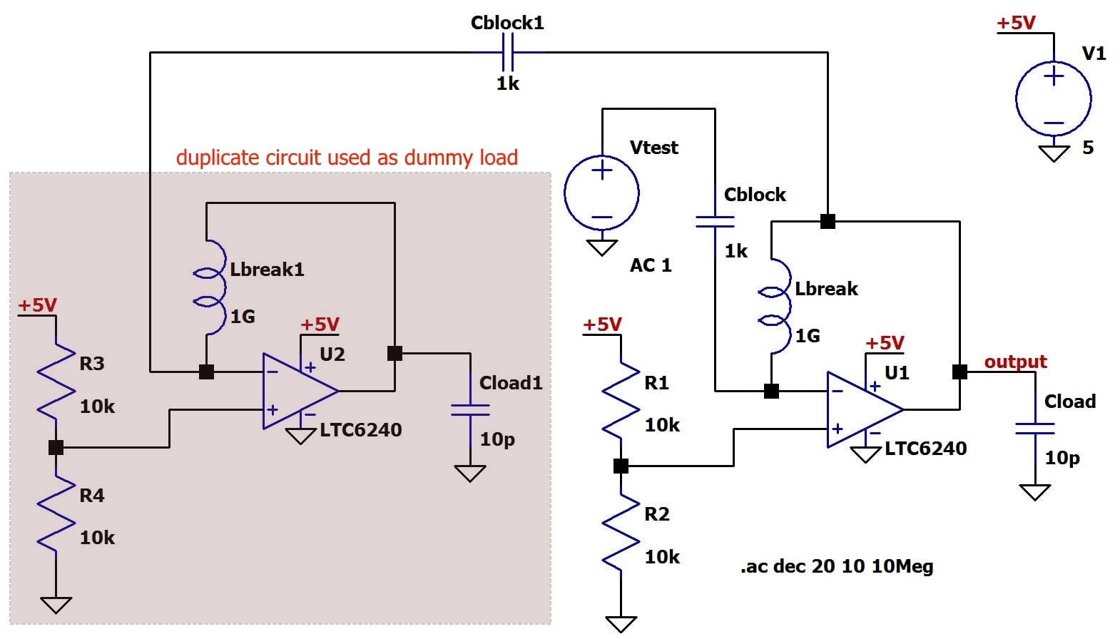
As you can see, the original feedback node is connected to the termination node through another large capacitor, in order to allow AC interaction while preserving DC bias conditions.

Now we are ready to simulate. All we need to do is plot V_output.

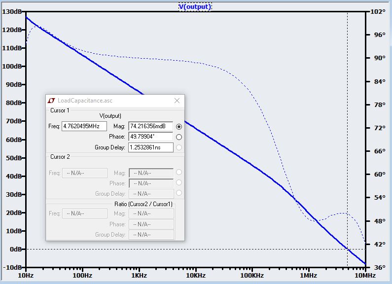
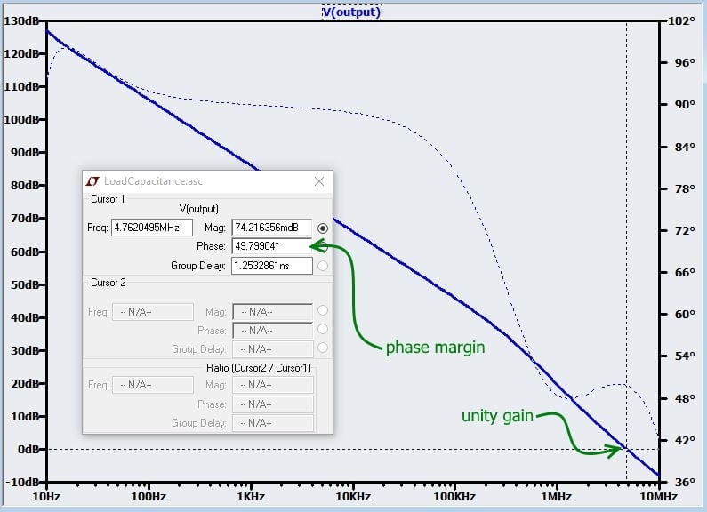
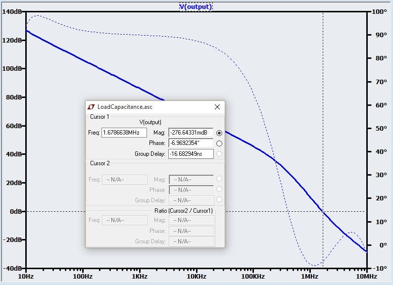
Recall that the break-the-loop method results in Aβ = -output. The negative sign corresponds to a 180° phase shift, and this turns out to be quite handy: the phase starts at 180° and approaches zero, meaning that phase margin is measured relative to 0° instead of 180°. Consequently, in this plot of V_output, if you move the cursor to the unity-gain frequency, the value given in the “Phase” box is the phase margin:

As expected, this internally compensated op-amp is thoroughly stable with such a small amount of load capacitance. But eventually we decide that our voltage reference needs some additional bypassing, so we add a 1 nF capacitor to the output of the op-amp (don’t forget to change the load capacitor in the duplicate circuit). Here is the new plot of -Aβ.

Now we have a problem. The phase margin has decreased past 0°, meaning that the circuit is now completely unstable (rather than merely not sufficiently stable). There are various techniques for increasing the stability of large-capacitive-load op-amp circuits; this expansive topic is beyond the scope of this article. Here we are focusing on stability analysis, so we will simply demonstrate the effect of one common, straightforward remedy: inserting a series resistor between the op-amp output and the load capacitor. The resistor creates a zero in the feedback transfer function, and the phase shift from this zero compensates for some of the problematic phase shift generated by the pole. The resistor should be sized so that the zero frequency is low enough to allow the phase to adequately recover. For this circuit, we can size the resistor according to information given in the datasheet for the LTC6240:

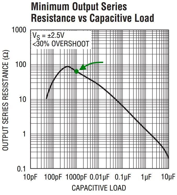
These values are for 30% overshoot, but we want something closer to 20% overshoot, so we’ll try 90 Ω:

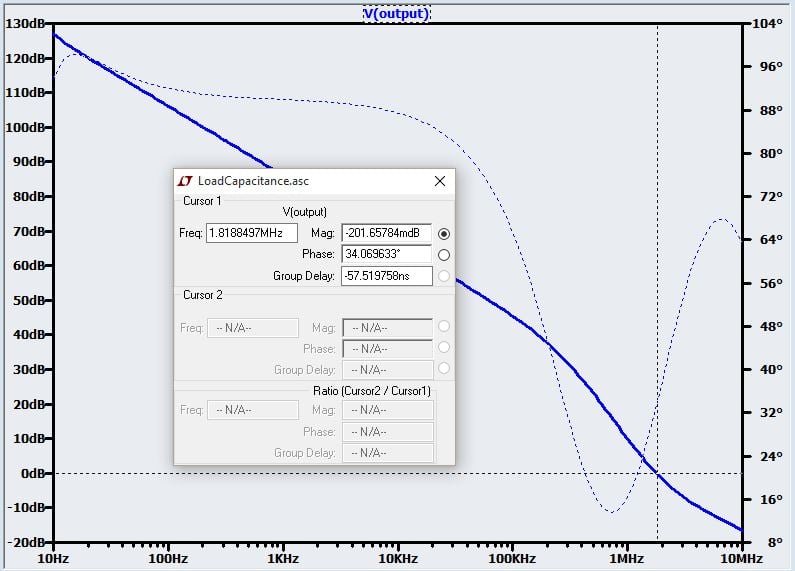
Now we have a phase margin of 34°, which is a little low but probably adequate. It takes about 130 Ω of series resistance to bring the phase margin up to 45°.

Conclusion

You now have in your analytical toolbox a simulation technique that can provide accurate, convenient stability information for a wide variety of negative-feedback circuits, from simple op-amp buffers to complex discrete-transistor amplifier topologies. In the next article we will conclude this series by exploring stability via time-domain, rather than frequency-domain, simulations.

Next Article in Series: Negative Feedback, Part 10: Stability in the Time Domain