Pole Splitting in Electronics

Learn how pole splitting arises as the byproduct of Miller frequency compensation.

Pole splitting arises most famously in connection with Miller frequency compensation, where placing a capacitor across an inverting gain stage causes the poles associated with that stage’s input and output ports to split into opposite directions in the s plane, the former shifting to a lower frequency, and the latter shifting to a higher frequency. A byproduct of Miller compensation is the creation of a right half-plane zero (RHPZ).

To illustrate, let’s start out with the basic gain stage of Figure 1, where the dependent source $$G_mV_1$$ models gain, and the $$R_1-C_1$$ and $$R_2-C_2$$ networks model the input-port and the output-port poles.  

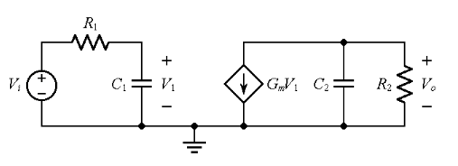
Figure 1. AC model of a gain stage.

By inspection,

$$V_1 =\frac{1/(sC_1)}{R_1+1/(sC_1)}V_i=\frac{1}{1+sR_1C_1}V_i \; \; \; \; V_o = - G_{m}V_{1} (R_2\parallel\frac{1}{sC_2} ) = \frac{-G_{m}R_2}{1+sR_2C_2}V_1$$

Equation 1

where s is the complex frequency. Eliminating $$V_1$$, we express the stage’s gain a(s) in the insightful form

$$a(s) =\frac{V_o}{V_i}=\frac{a_0}{(1+s/\omega _{10})(1+s/\omega_{20})}$$

Equation 2

where

$$a_0 = -G_mR_2$$

Equation 3

is the stage’s dc gain, which is negative, and

$$\omega_{10} = \frac {1}{R_1C_1} \; \; \; \; \; \; \; \;  \omega_{20} = \frac {1}{R_2C_2}$$

Equation 4

are the angular frequencies associated with the input-port and output-port poles. (Recall that the angular frequency ω, in radians/sec, and the frequency f, in Hertz, are related as ω = 2πf). 

The denominator of a(s) vanishes for $$s = –\omega_{10}$$ and $$s = –\omega_{20}$$, which are aptly called the poles of a(s) because they cause a(s) to blow up to infinity. In this case, both poles lie on the negative real axis of the s plane.

Let us now connect the capacitor $$C_f$$ across the gain stage as in Figure 2, and let us recalculate the gain a(s). 

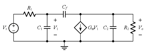
Figure 2.  AC model of a gain stage with $$C_f$$ present.

Applying KCL at the node to the left of $$C_f$$ gives

$$\frac{V_i-V_1}{R_1} = \frac {V_1}{1/(sC_1)}+\frac{V_1-V_o}{1/(sC_f)}$$

Equation 5a

Likewise, KCL at the node to the right of $$C_f$$ gives 

$$\frac{V_1-V_o}{1/(sC_f)} = G_mV_1 + \frac{V_o}{R_2}+\frac {V_o}{1/(sC_2)}$$

Equation 5b

Eliminating $$V_1$$ and solving for the ratio $$V_o/V_i$$ we get, after suitable algebraic manipulations, 

$$a(s) = \frac{V_o}{V_i} = a_0 \frac{1-sC_f/G_m}{1+s\left\{R_1[C_1+C_f(1+G_mR_2)]+R_2(C_f+C_2)\right\}+s^2R_1R_2(C_1C_f+C_1C_2+C_fC_2)}$$

Equation 6

with $$a_0$$ as in Equation 3.  It is fair to say that the above expression doesn’t provide a tremendous amount of insight, yet we can still glean some interesting peculiarities.  

• Despite the presence of three reactive elements, the circuit is only of the second-order type. This is so because the capacitors form a loop, so once we know the voltages across two of them, the voltage across the third is also known, by KVL, so we have only two degrees of freedom.  
• The numerator vanishes for $$1 – sC_f/G_m = 0$$, indicating a gain of zero for $$s = ω_0$$, where 
   

$$\omega_0 = \frac {G_m}{C_f}$$

Equation 7

and $$\omega_0$$ is aptly referred to as a zero frequency. 

Physically, the current transmitted via $$C_f$$ towards the output node splits among $$R_2$$, $$C_2$$, and the dependent source.  If we adjust s so that the current sourced by $$C_f$$ equals that sunk by the dependent source, then none will go to $$R_2$$ and $$C_2$$, thus implying $$V_o$$ = 0.  When this happens, we have $$(V_1 – 0)/[1/(sC_f)] = G_mV_1,$$ or $$sC_f = G_m$$, or $$s = G_m/C_f = ω_0$$.  This zero lies on the positive real axis of the s plane, so it is known as a right half-plane zero (RHPZ). 

Based on the above observations, we stipulate a gain expression of the more insightful type 

$$a(s) =\frac {V_o}{V_i}=a_0\frac {1-s/\omega_0}{(1+s/\omega_1)(1+s/\omega_2)}$$

Equation 8

with $$a_0$$ as in Equation 3, and $$ω_0$$ as in Equation 7. Our next task is to seek possibly insightful expressions for the pole frequencies $$\omega_1$$ and $$\omega_2$$.  Given the negative-feedback action provided by $$C_f$$, we expect these frequencies to be quite different from $$\omega_{10}$$ and $$\omega_{20}$$ of Equation 4, where subscript zero was meant to signify “with $$C_f$$ = 0.” In particular, being already familiar with the Miller effect, we anticipate a dominant pole on the order of 

$$\omega_1\cong \frac {1}{R_1[C_1+C_f(1+G_mR_2)]}$$

Equation 9

and such that $$\omega_1 << \omega_2$$.  This last condition allows us to make the following approximation:

$$\frac{1-s/\omega_0}{(1+s/\omega_1)(1+s/\omega_2)}=\frac{1-s/\omega_0}{1+s/\omega_1 +s/\omega_2+s^2/(\omega_1 \omega_2)}\approx\frac{1-s/\omega_0}{1+s/\omega_1 +s^2/(\omega_1 \omega_2)}$$

Equation 10

Equating the coefficients of s in the denominators of Equations 6 and 10, we easily find 

$$\omega_1 = \frac {1}{R_1[C_1+C_f(1+g_mR_2+R_2/R_1)]+R_2{C_2}}$$

Equation 11

Considering that both denominators in Equations 9 and 11 are usually dominated by the Miller capacitance $$C_M = C_f(1 + G_mR_2)$$, we have a good reason to trust that the approximation of Equation 9 is a fairly good one.

Equating the coefficients of $$s^2$$ in the denominators of Equations 6 and 10, we get

$$\omega_1\omega_2 = \frac{1}{R_1R_2[C_f(C_1+C_2)+C_1C_2]}$$

Equation 12

indicating that for a given $$C_f$$, the product $$\omega_1\omega_2$$ is constant, so the downshift $$\omega_{10}$$ → $$\omega_{1}$$ must be accompanied by an upshift $$\omega_{20} \rightarrow  \omega_{2}$$. 

Pole-Splitting in PSpice

Let us use PSpice to observe the pole-splitting phenomenon. Consider Figure 3, below.

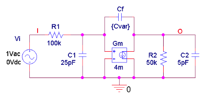
Figure 3. PSpice circuit to plot pole splitting for $$C_f = 2 pF$$.

With the component values shown, we have (by Equation 4), $$\omega_{10} = 1/(100 \times10^3 \times 25 \times10^{–12})$$ = 400 krad/s and $$\omega_{20}$$ = 4.0 Mrad/s, corresponding to the frequencies 

$$f_{10} = 63.66 kHz \; \; \; \; \; \; \; \; f_{20} = 636.6 kHz$$

Equation 13

which are separated by a decade. By Equation 11 we have

Note, incidentally, that had we used Equation 9, we would have gotten $$\omega_1$$ = 23.42 krad/s, a fairly good approximation. By Equation 12 we have

$$\omega_2=\frac{1/23.23 \times 10^3}{10^5\times50\times10^3[2\times10^{-12}(25+5)10^{-12}+25\times5\times10^{-24}]}=46.40 \; Mrad/s$$

Finally, Equation 7 gives $$\omega_0 = 4 \times 10^{–3}/(2 \times 10^{–12})$$ = 2.0 Grad/s. The above data yield the frequencies

f₁ = 3.70 kHz        f₂ = 7.38 MHz        f₀ = 318 MHz                

Our findings are confirmed by the plots of Figure 4. 

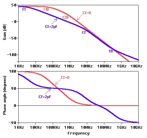
Figure 4.  Gain magnitude and phase plots for the PSpice circuit of Figure 3.

In summary, the presence of C_f has a triple effect:

1. It downshifts the first pole frequency by a factor of 63.66/3.70 = 17.2.
2. It upshifts the second pole frequency by a factor of 7,380/636.6 = 11.6.
3. It establishes a transmission zero at 318 MHz. 

The pole/zero situation in the s plane is depicted in Figure 5.

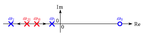
Figure 5. S-plane illustration (not to scale) of pole splitting as well as RHPZ creation.

The Right Half-Plane Zero (RHPZ)

Let us conclude by taking a closer look at the right half-plane zero (RHPZ), which will be referenced abundantly in the next article on stability in the presence of a RHPZ. 

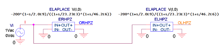
Figure 6. PSpice circuit to contrast a RHPZ and a LHPZ.

Looking first at the $$C_f$$ = 0 plots of Figure 4, we note that from $$f_{10}$$ to $$f_{20}$$ magnitude rolls off at the rate of –20 dB/dec, and past $$f_{20}$$ at the rate of –40 dB/dec. The corresponding phase angle swings from 180° (due to the fact that $$a_0$$ is negative) to 90°, and then from 90° to 0°.  

Turning next to the $$C_f$$ = 2 pF plots, we note that from $$f_1$$ to $$f_2$$ magnitude rolls off at a rate of –20 dB/dec, from $$f_2$$ to $$f_0$$ at a rate of –40 dB/dec, and past $$f_0$$ again at a rate of –20 dB/dec. The corresponding phase angle swings from 180° to 90° and from 90° to 0° because of the pole frequencies $$f_1$$ and $$f_2$$ , and then from 0° to –90° because of the RHPZ frequency $$f_0$$. In other words, a RHPZ introduces a phase delay just like an ordinary left half-plane pole! This delay may destabilize a negative-feedback circuit containing a RHPZ around the loop. (For more information on this issue, please refer to The Right Half-Plane Zero and Its Effect on Stability.)   

Put another way, the gain stage acts as an inverting amplifier for $$f < f_0$$, but as a noninverting amplifier for $$f > f_0$$, thus turning the overall feedback from negative to positive, and possibly destabilizing the loop.

To further evidence similarities and differences between a RHPZ and a LHPZ, consider the expressions

$$a_{RHPZ} = a_0 \frac{1-s/\omega_0}{(1+s/\omega_1)(1+s/\omega_2)} \; \; \; \; \; \; \; \; \; \; a_{LPHZ}= a_0 \frac{1+s/\omega_0}{(1+s/\omega_1)(1+s/\omega_2)}$$

Equation 14

which we are going to simulate via PSpice using the parameter values of Equation 14. To find expressions for magnitudes and phase angles in terms of frequency ω, we let s → jω.  Then we write

$$Mag[a_{ORHPZ}]= Mag[a_{OLPHZ}] = \left | a_o \right |\sqrt{\frac{1+(\omega/\omega_0)^2}{(1+(\omega/\omega_1)^2)\times(1+(\omega/\omega_2)^2)}}$$

$$Ph[a_{ORPHZ}]=180^\circ - tan^{-1} (\omega/\omega_0)- tan^{-1}(\omega/\omega_1)- tan^{-1}(\omega/\omega_2)$$

$$Ph[a_{OLPHZ}]=180^\circ + tan^{-1} (\omega/\omega_0)- tan^{-1}(\omega/\omega_1)- tan^{-1}(\omega/\omega_2)$$

Magnitudes are the same because $$Mag[a \pm jb] = \sqrt{(a^2 + b^2)}$$. However, the phase angles differ because $$Ph[a \pm jb] = \pm tan^{-1} (b/a)$$. Magnitude similarity as well as phase-angle difference are evidenced in Figure 7. 

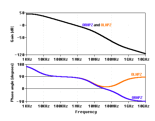
Figure 7. Gain magnitude and phase plots for the PSpice circuits of Figure 6.

It is important to realize that phase-margin estimations via the rate-of-closure (ROC) are not applicable in the present case because a system with a RHPZ is not a minimum-phase system.

References

1. http://online.sfsu.edu/sfranco/BookAnalog/AnalogJacket.pdf

If you enjoyed this article, let us know in the comments below!