Miller Frequency Compensation: How to Use Miller Capacitance for Op-Amp Compensation

Miller capacitance is commonly used in a method for operational amplifier frequency compensation.

In my previous articles, we discussed op-amp frequency compensation and one compensation method via shunt capacitance.

The frequency compensation technique in widest use today is called Miller frequency compensation, which we will explore in this article.

 

What Is Miller Compensation?

Miller compensation is a technique for stabilizing op-amps by means of a capacitance C_ƒ connected in negative-feedback fashion across one of the internal gain stages, typically the second stage.

 

Utilizing Miller Compensation

Using the PSpice circuit of Figure 1, which was introduced in the previous article on frequency compensation, we obtain the magnitude/phase plots of Figure 2, showing that the presence of C_ƒ causes the pole frequencies to split apart. Specifically, the higher the value of C_ƒ is, the further apart the pole frequencies and, hence, the wider the intermediate frequency region of phase shifts close to –90°. 

 

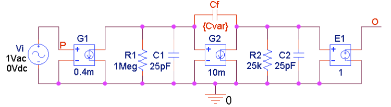
Figure 1. PSpice circuit to plot the open-loop gain magnitude and phase for different amounts of Miller compensation.

 

Figure 3 provides an expanded view of the region of the crossover frequencies to facilitate a visual estimation of phase margins. Given a magnitude curve, (1) we identify the position of its crossover frequency ƒ_x on the 0-dB axis, (2) then we turn to the corresponding phase curve below, and (3) finally we read the phase shift ɸ_x at the right. Then the phase margin is ɸ_m = 180° + ɸ_x. For instance, for C_ƒ = 8 pF, corresponding to the 4^th curve after the C_ƒ = 0 curve, we estimate ɸ_x ≈ –120°, so ɸ_m ≈ 60°. 

Conversely, we can visually come up with a rough estimation for the value of C_ƒ required for a given ɸ_m, and then refine C_ƒ using the trial-and-error approach via PSpice. As an example, for ɸ_m ≈ 65.5°, which marks the onset of AC peaking, the above procedure yields C_ƒ = 9.90 pF. The corresponding pole frequencies are measured to be 63.4 Hz and 12.2 MHz.

 

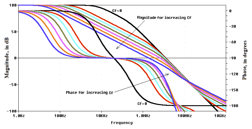
Figure 2.  Magnitude/phase plots of the circuit of Figure 1 for different values of the compensating capacitance C_ƒ: 0, 1 pF, 2 pF, 4 pF, 8 pF, 16 pF, and 32 pF. 

 

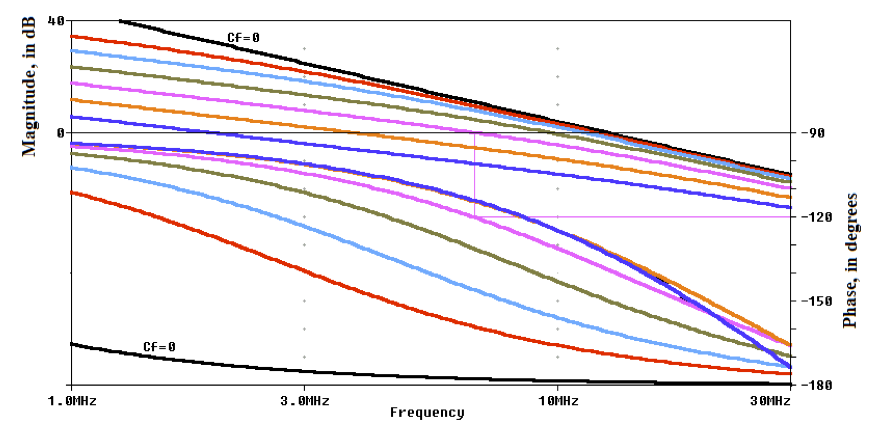
Figure 3.  Expanded view of the area of the crossover frequencies of Figure 2.

Using the PSpice circuit of Figure 4 with C_ƒ = 9.90 pF to provide Miller compensation, we get the plots of Figure 5, all of which are exempt from peaking!

 

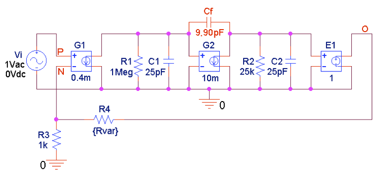
Figure 4.  PSpice circuit to plot closed-loop gains in 20-dB steps determined by R₄.

 

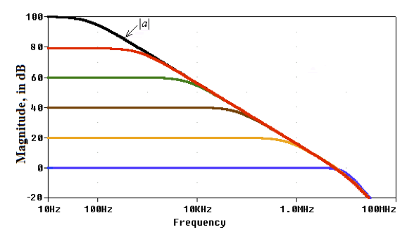
Figure 5.  Stepped responses of the PSpice circuit of Figure 4 after Miller compensation with C_ƒ = 9.90 pF.

The Miller Effect for Capacitance

In the previous article on frequency compensation, we found that making the first pole dominant required a shunt capacitance of tens of nanofarads. Miller compensation, on the other hand, requires only picofarads. 

How come? The answer is provided by the Miller effect.

The Miller effect refers to the increase in equivalent capacitance that occurs when a capacitor is connected from the input to the output of an amplifier with large negative gain.

This concept is illustrated in Figure 6 for the capacitance case. 

 

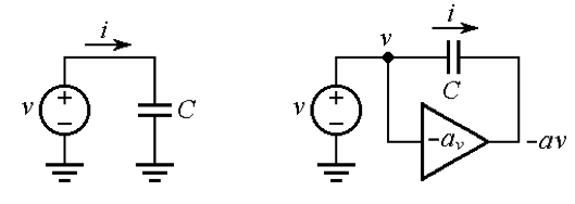
(a)                                                                                        (b)

Figure 6. Illustrating the Miller effect for capacitance. 

 

In response to an applied voltage v, as in Figure 6(a), a capacitor C responds with the current $$i = C\frac{dv}{dt}$$. If we now connect the same capacitor C in feedback fashion across an inverting voltage amplifier with gain –a_v, as depicted in Figure 6(b), then the current becomes

 

$$i=C\frac{d[v-(-a_{v}v)]}{dt}=C\frac{dv(1+a_{v})}{dt}=C_{M}\frac{dv}{dt}$$

Equation 1

 

Miller Capacitance

The quantity C_M in Equation 1 is referred to as the Miller capacitance and is calculated as follows

 

$$C_{M}=(1+a_{v})C$$

Equation 2. The Miller capacitance

 

In words, the feedback capacitance C reflected to the input, gets multiplied by 1 + a_v. This makes it possible to synthesize large capacitances with relatively small physical capacitors.

With reference to the PSpice circuit of Figure 4, we have

 

C_M = (1 + G_m2R₂)C_ƒ = (1 + 250)9.90 pF = 2.485 nF

 

The total capacitance seen by R₁ is C_total = C_M + C₁ = 2.51 nF, so the dominant pole frequency is 1/(2πR₁C_total) = 63.4 Hz, in agreement with the value measured above via PSpice. 

A systematic analysis of pole splitting, which is beyond the scope of this article, indicates that with Miller compensation, the new pole frequencies are approximately related to the originals ƒ₁ and ƒ₂ as

 

$$f_{1(new)}≈f_{1}\frac{1}{G_{m2}R_{2}}\times \frac{C_{1}}{C_{f}}$$

$$f_{2(new)}≈f_{2}\times G_{m2}R_{2}\times \frac{C_{f}}{C_{1}+C_{f}(1+\frac{C_{1}}{C_{2}})}$$

Equation 3

 

where ƒ₁ = 1/(2πR₁C₁) and ƒ₂ = 1/(2πR₂C₂). Since ƒ_2(new) is directly proportional andƒ_1(new) is inversely proportional to the second-stage gain G_m2R₂, it is apparent that the larger this gain is, the wider the pole separation for a given C_ƒ. This is highly desirable because with a sufficiently high gain, the required C_ƒ for a given phase margin can be kept small enough (not more than a few tens of picofarads) so it can be fabricated on-chip. Moreover, the smaller C_ƒ is, the faster the op-amp dynamics, since the open-loop bandwidth, slew rate, and full power bandwidth are all inversely proportional to C_ƒ.

A Bit of History

The first integrated circuit (IC) op-amp to incorporate full compensation was the venerable µA741 op-amp (Fairchild Semiconductor, 1968), which used a 30-pF on-chip capacitor for Miller compensation. The open-loop gain characteristics of the µA741 macro model available in PSpice are shown in Figure 7.

 

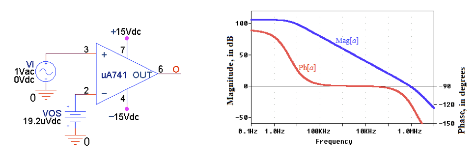
Figure 7.  Plotting the open-loop gain a of the µA741 op-amp.

 

The magnitude curve crosses the 0-dB axis at ƒ_x = 888.2 kHz, where Ph[a] = –117°, for a phase margin of ɸ_m ≈ 63°.  Things go as if the µA741 had a second pole at ƒ₂ = tan(ɸ_m)ƒ_x = 1.743 MHz.

Before the advent of the µA741, all IC op-amps had to be compensated externally by the user.  A popular uncompensated contemporary of the µA741was the LM301 (National Semiconductor), which offered the user three compensation options to meet different objectives: the single-pole compensation, the double-pole compensations, and the feedforward compensation. 

Even though the µA741 offered far less compensation flexibility than the LM301, the mA741 took off meteorically, most likely because many users were relieved of the oft-unpleasant task of providing external compensation without having a thorough understanding of its inner workings.

 

---

 

In the next article, we'll look at decompensated operational amplifiers.