Facebook
 Google
 GitHub
 Linkedin
Shunt Capacitance Compensation in Operational Amplifiers
In this article, we'll discuss how shunt capacitance can be used to achieve frequency compensation in op-amps and we'll also see why this is not the preferred technique.
In this article, we'll discuss how shunt capacitance can be used to achieve frequency compensation in op-amps and we'll also see why this is not the preferred technique.
In a recent article on the frequency compensation of operational amplifiers, we discussed what the concept of frequency compensation is and how we can evaluate an example circuit's stability. We concluded that article by addressing the concept of dominant-pole compensation and how it was necessary to modify the open-loop gain to allow a profile that is dominated by a single pole.
Here, we will show a method for achieving this, known as shunt capacitance. Shunt capacitance compensation involves intentionally adding capacitance in parallel with the existing capacitance of one of the circuit's nodes.
Compensation via a Shunt Capacitor
A brute-force way of making a pole dominant is to intentionally add capacitance to the node responsible for the lowest pole frequency.
In the previous article, we introduced the two-pole op-amp model of Figure 1 below, where f1 is the lowest pole frequency.
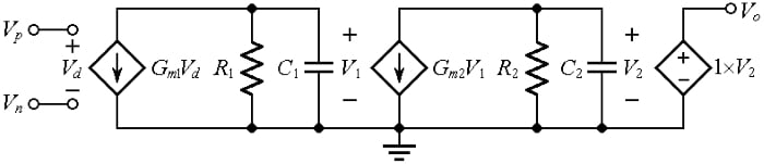
Figure 1. Approximate AC model of an op-amp.
We then used the PSpice circuit of Figure 2 to generate the plots of Figure 3.
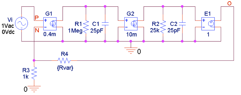
Figure 2. PSpice circuit to plot closed-loop gains in 20-dB steps determined by R4.
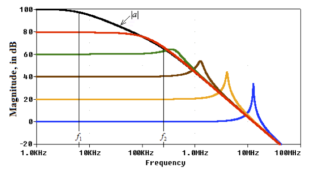
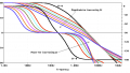
Figure 3. Closed-loop gains of the circuit of Figure 2 for different amounts of feedback.
These plots indicate that the op-amp needs to be frequency compensated to prevent the gain peaking occurring especially at the lower closed-loop gains.
Once we decide where to position the crossover frequency ƒx for unity-gain operation, we find the new value of ƒ1 by exploiting the constancy of the gain-bandwidth product of the compensated gain, or a0׃1(new) = 1׃x, thus giving
$$f_{1(new)}=\frac{f_{x}}{a_{0}}$$
Equation 1
A good starting point is to impose ƒx = ƒ2 because it is easy to visualize geometrically.
For the circuit of Figure 2, we get ƒ1(new) = ƒ2/a0 =2.546 Hz, and we find the required value of the compensating capacitance Cc (to be placed in parallel with C1) by letting 1/[2πR1(C1 + Cc)] = ƒ1(new), which gives Cc = 62.51 nF.
Rerunning the circuit of Figure 2, but with Cc added as in Figure 4 (below), we obtain the plots of Figure 5. Except for the unity-gain case, all profiles are now exempt from peaking because each enjoys a 90° phase margin.
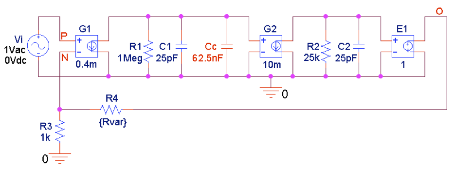
Figure 4. PSpice circuit to plot closed-loop gains in 20-dB steps after shunt-capacitance compensation.
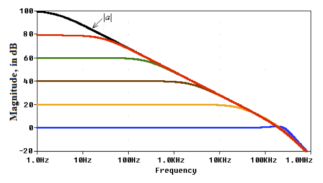
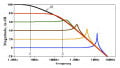
Figure 5. Closed-loop gains of the circuit of Figure 4.
Comparing Figure 5 against Figure 3, we observe that the price for getting rid of peaking is a much-reduced open-loop bandwidth. In fact, the open-loop bandwidth ƒ1 is reduced from 6.366 kHz to 2.546 Hz.
The slight amount of peaking by the unity-gain response is due to the fact that by letting ƒx = ƒ2 we are imposing a ROC of 30 dB/dec, implying a phase margin of ɸm ≈ 45°. If a higher ɸm is desired, then ƒx must be placed below ƒ2 such that
$$f_{x}=\frac{f_{2}}{tanɸ_{m}}$$
Equation 2
For instance, for ɸm ≈ 65.5°, which marks the onset of peaking, we need to impose ƒx = ƒ2/(tan 65.5°) = ƒ2/2.194. Consequently, we need Cc = 62.51×2.194 = 137 nF, and we get ƒ1(new) = 2.546/2.194 =1.16 Hz.
It's important to understand that shunt-capacitance compensation is attractive from a pedagogical standpoint, but that’s about all. Not only does it cause a dramatic bandwidth reduction, but it also slows down other dynamics such as the slew rate and the full-power bandwidth. We will be discussing a more practical and widely-used method in the next article on Miller frequency compensation.
Now that you have an understanding of one method of achieving frequency compensation in an op-amp, let's talk about a much better alternative, Miller compensation, which is discussed in the next article.
Related Content