Facebook
 Google
 GitHub
 Linkedin
The Right Half-Plane Zero and Its Effect on Stability
In this article, we will discuss the right half-plane zero, a byproduct of pole splitting, and its effects on stability.
In this article, we will discuss the right half-plane zero, a byproduct of pole splitting, and its effects on stability.
A previous article discussed Miller frequency compensation using the three-stage op-amp model of Figure 1 as a vehicle.

Figure 1. Ac model of a Miller compensated three-stage op-amp.
This type of compensation benefits from pole splitting, but it also creates a right half-plane zero (RHPZ) as a notorious byproduct.
The linearized magnitude Bode plot of Figure 2 shows the relevant parameters of the open-loop gain $$a(jf) = V_o/V_d$$.

Figure 2. Gain magnitude profile of a Miller compensated op-amp.
These parameters include:
- The dc gain $$a_0$$
- The pole-frequency pair $$f_1$$ and $$f_2$$, with $$f_1$$ being the dominant pole
- The transition frequency $$f_t$$ at which gain crosses the 0 dB axis
- The zero frequency $$f_0$$ associated with the RHPZ
Finally, it also shows the gain-bandwidth product,
$$GBP = a_0 \times f_1$$
Equation 1
whose value is approximately constant from about a decade after $$f_1$$ to about a decade before $$f_2$$.
For the circuit example of Figure 3, it was found that a compensating capacitance Cf = 9.9 pF ensures unity-gain voltage-follower operation with a phase margin $$\phi_m = 65.5 ^{\circ}$$, so chosen because it marks the onset of gain peaking.
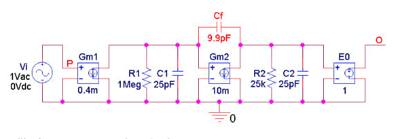
Figure 3. Using PSpice to illustrate an actual example.
The salient features of this amplifier are shown via the magnitude and phase plots of Figure 4.
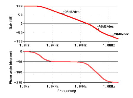
Figure 4. Gain magnitude and phase for the circuit of Figure 3.
Cursor measurements give: $$a_0 = 10^5 V/V$$, $$f_1 = 63.4 Hz$$, $$GBP = 6.34 MHz$$, $$f_t = 5.87 MHz$$, and the phase angle $$Ph[a(jf_t)] = –114.5^{\circ}$$.
(Note that the transition frequency $$f_t$$ is a bit less than the GBP because the magnitude curve starts to bend downward a bit before $$f_2$$.)
The Right Half-Plane Zero (RHPZ)
The RHPZ has been investigated in a previous article on pole splitting, where it was found that
$$f_0=\frac{1}{2\pi} \frac{G_{m2}}{C_f}$$
Equation 2
so the circuit of Figure 3 has $$f_0 = 10 \times 10^{-3} /(2\pi \times 9.9 \times10^{-12}) = 161 MHz$$. The most salient feature of a RHPZ is that it introduces phase lag, just like the conventional left half-plane poles (LHPPs) $$f_1$$ and $$f_2$$ do. This lag tends to erode the phase margin for unity-gain voltage-follower operation, possibly leading to instability. (Conversely, a LHPZ introduces phase lead, which tends to ameliorate the phase margin.) In Figure 2 the phase contribution by the RHPZ at the transition frequency is $$\Delta \phi = - tan^{-1}(f_t/f_0)$$, which, for the circuit of Figure 3, amounts to $$\Delta \phi= – tan^{-1}(5.87/161) \cong –2.1^\circ$$. This is so small that in order to keep things simple, the RHPZ was deliberately omitted from the discussion of Miller compensation.
Now we wish to take a closer look at how the RHPZ affects stability. Let us start out with the dominant pole, which is given by Equation 11 of the aforementioned article on pole splitting:
$$\omega _1 =\frac {1}{R_1[C_1+C_f(1+G_{m2} R_2 +R_2/R_1)]+R_2C_2}$$
Equation 3
Retaining only the dominant portion, we approximate as
$$\omega _1 \cong \frac {1}{R_1C_f G_{m2} R_2}$$
Equation 4
Using Equations 1 and 4, along with $$a_0 = G_{m1}R_1G_{m2}R_2$$, we write
$$GBP \cong G_{m1}R_1G_{m2}R_2 \frac {1/2\pi}{R_1C_fG_{m2}R_2} = \frac {1}{2\pi} \frac {G_{m1}}{C_f}$$
Equation 5
Combining Equations 2 and 5 gives
$$f_0 \cong GBP \frac {G_{m2}}{G_{m1}}$$
Equation 6
The higher the ratio $$G_{m2}/G_{m1}$$, the lower the amount of phase-margin erosion by the RHPZ. In Figure 3, $$G_{m2}/G_{m1} = 10/0.4 = 25$$, yielding an erosion of $$\Delta \phi = –tan^{–1}(1/25) \cong–2.3^{\circ}$$, fairly close to –2.1° calculated earlier. In the 741 op-amp (here, you may reference my book on analog circuit design), $$G_{m2} \cong 6.25 mA/V$$ and $$G_{m1} \cong 0.183 mA/V$$, corresponding to a phase-margin erosion of $$\Delta \phi \cong –1.7^{\circ}$$.
There are circuits in which the condition $$G_{m2}/G_{m1}$$ >> 1 does not hold. The two-stage CMOS op-amp is a notorious example because it is usually implemented with $$G_{m2}/G_{m1} = 2$$. The phase-margin erosion is now $$\Delta \phi \cong –tan^{–1}(1/2) \cong –27^{\circ}$$, which makes it difficult, if not impossible, to ensure adequately safe phase margins.
This is confirmed by the circuit of Figure 5 and the corresponding plots of Figure 6.
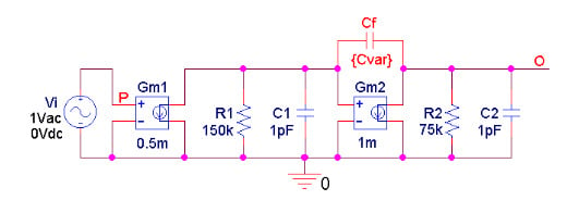
Figure 5. PSpice circuit for an amplifier with $$G_{m2}/G_{m1}= 2$$.
It is apparent that the zero frequencies of the magnitude curves are just too close to the corresponding transition frequencies to allow the designer much flexibility in achieving acceptable phase margins.

Figure 6. Gain magnitude and phase for the circuit of Figure 5 for different values of the compensating capacitance $$C_f$$: 0, 1 pF, 2 pF, 4 pF, 8 pF, 16 pF, and 32 pF.
Relocating the RHPZ
One way to overcome the above difficulties is to relocate the RHPZ by placing a resistance $$R_f$$ in series with $$C_f$$, as depicted in Figure 7.
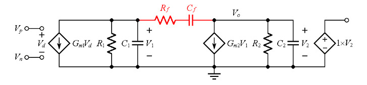
Figure 7. Relocating the RHPZ by means of $$R_f$$.
To see how this happens, note that in order to drive $$V_o$$ to zero, the current drawn by the dependent source $$G_{m2}V_1$$ must equal the current supplied by $$V_1$$ via the $$R_f-C_f$$ network. Using KCL and the generalized Ohm’s law, we thus impose
$$\frac {V_1 - 0}{R_f +1/(sC_f)} = G_{m2}V_1$$
Equation 7
where s is the complex frequency. The value of s satisfying the above equality is the zero frequency $$\omega_0$$,
$$\omega _0 = \frac {1}{(1/G_{m2}-R_f)C_f}$$
It is apparent that by proper choice of $$R_f$$ we can relocate the zero virtually anywhere on the x-axis of the complex plane. A good choice is to impose $$R_f = 1/G_{m2}$$, which will move the zero to infinity, completely out of the way! For our amplifier example, $$R_f = 1/10^{–3} = 1 k\Omega $$.
Using the PSpice circuit of Figure 8, it was found by trial and error that to achieve a phase margin of $$\phi_m = 65.5^{\circ}$$, which marks the onset of gain peaking, the circuit requires $$C_f = 2.46 pF$$.
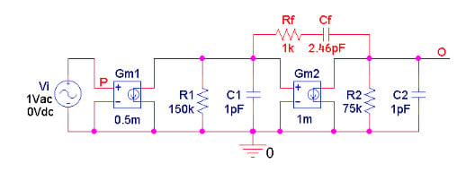
Figure 8. PSpice circuit with $$R_f = 1/G_{m2}$$ to send the RHPZ to infinity.
This is confirmed by the magnitude/phase plots of Figure 9.
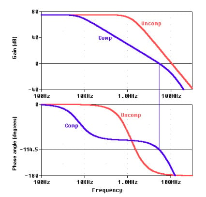
Figure 9. Gain magnitude and phase for the circuit of Figure 8. The phase margin for the compensated case is $$\phi_m = 180^{\circ} – 114.5^{\circ} = 65.5^{\circ}$$.
For comparison, also shown are the curves for the uncompensated case ($$R_f = \infty$$ and $$C_f = 0$$), which indicate a phase-margin approaching zero.
Now let us turn to Figure 10 to observe how the circuit of Figure 8 responds in negative-feedback operation as a voltage follower.
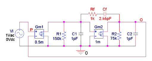
Figure 10. Configuring the amplifier of Figure 8 as a unity-gain voltage follower.
The results, shown in Figure 11, indicate that without compensation ($$R_f = \infty$$ and $$C_f = 0$$) the gain exhibits an intolerable amount of peaking, due to its phase margin being close to zero, as per the phase plot of Figure 9. On the other hand, full compensation ($$R_f = 1 k\Omega$$ and $$C_f = 2.46 pF$$) gets rid of peaking.
Also shown for comparison is what happens if $$R_f$$ is shorted out to leave in place only $$C_f$$ for frequency compensation. It turns out that the phase margin drops from 65.5° to 38.8°, indicating a peaked response. Not as bad as in the uncompensated case, but still not as good as in the fully compensated case.

Figure 11. Closed-loop gain of the voltage follower of Figure 10.
Active Elimination of the RHPZ
A clever way to get rid of the RHPZ altogether is to interpose a voltage follower between the output node $$V_o$$ and the compensation capacitance $$C_f$$.
As depicted in Figure 12 for the case of a two-stage CMOS op-amp, the source follower $$M_f$$ will provide $$C_f$$ with whatever ac current it takes to sustain the Miller effect.
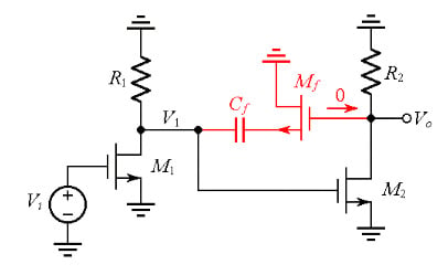
Figure 12. AC model of a two-stage CMOS op-amp using the source follower $$M_f$$ to prevent current transmission to the output node, and thus inhibit the formation of the RHPZ.
However, none of this ac current will be transmitted to the output node (recall that the gate current is zero), thus preventing the formation of the RHPZ!
References
- Analog Circuit Design: Discrete and Integrated by Sergio Franco