Understanding Poles and Zeros in Transfer Functions

This article explains what poles and zeros are and discusses the ways in which transfer-function poles and zeros are related to the magnitude and phase behavior of analog filter circuits.

In the previous article, I presented two standard ways of formulating an s-domain transfer function for a first-order RC low-pass filter. Let’s briefly review some essential concepts.

• A transfer function mathematically expresses the frequency-domain input-to-output behavior of a filter.
• We can write a transfer function in terms of the variable s, which represents complex frequency, and we can replace s with jω when we need to calculate magnitude and phase response at a specific frequency.
• The standardized form of a transfer function is like a template that helps us to quickly determine the filter’s defining characteristics.
• Mathematical manipulation of the standardized first-order transfer function allows us to demonstrate that a filter’s cutoff frequency is the frequency at which magnitude is reduced by 3 dB and phase is shifted by –45°.

 

Poles and Zeros

Let’s assume that we have a transfer function in which the variable s appears in both the numerator and the denominator. In this situation, at least one value of s will cause the numerator to be zero, and at least one value of s will cause the denominator to be zero. A value that causes the numerator to be zero is a transfer-function zero, and a value that causes the denominator to be zero is a transfer-function pole.

Let’s consider the following example:

 

$$T(s)=\frac{Ks}{s+\omega _{O}}$$

 

In this system, we have a zero at s = 0 and a pole at s = –ω_O.

Poles and zeros are defining characteristics of a filter. If you know the locations of the poles and zeros, you have a lot of information about how the system will respond to signals with different input frequencies.

The Effect of Poles and Zeros

A Bode plot provides a straightforward visualization of the relationship between a pole or zero and a system’s input-to-output behavior.

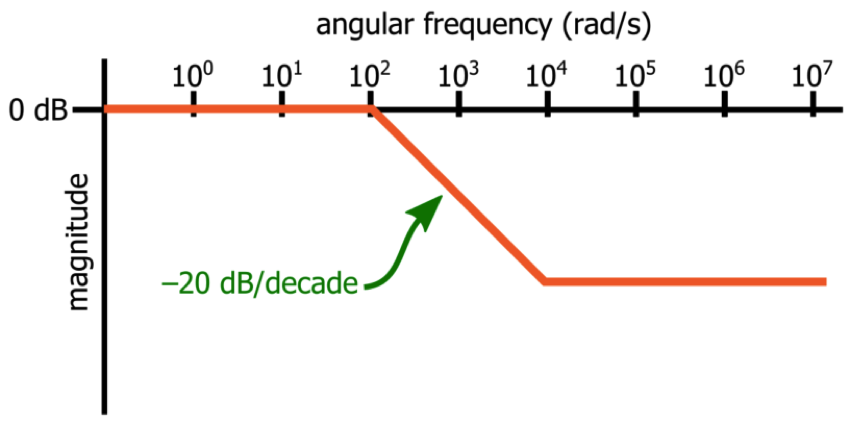
A pole frequency corresponds to a corner frequency at which the slope of the magnitude curve decreases by 20 dB/decade, and a zero corresponds to a corner frequency at which the slope increases by 20 dB/decade. In the following example, the Bode plot is the approximation of the magnitude response of a system that has a pole at 10² radians per second (rad/s) and a zero at 10⁴ rad/s.

 

Phase Effects

In the previous article, we saw that the mathematical origin of a low-pass filter’s phase response is the inverse tangent function. If we use the inverse tangent function (more specifically, the negative inverse tangent function) to generate a plot of phase (in degrees) versus logarithmic frequency, we end up with the following shape:

 

 

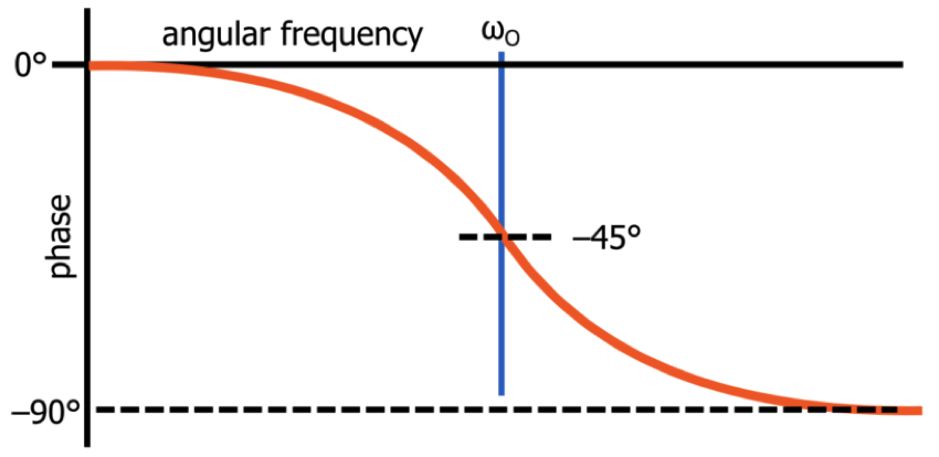
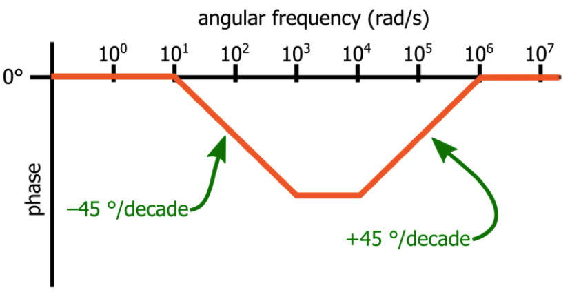
The Bode plot approximation for phase shift generated by a pole is a straight line representing –90° of phase shift. The line is centered on the pole frequency and has a slope of –45 degrees per decade, which means that the downward-sloping line begins one decade before the pole frequency and ends one decade after the pole frequency. The effect of a zero is the same except that the line has a positive slope, such that the total phase shift is +90°.

The following example represents a system that has a pole at 10² rad/s and a zero at 10⁵ rad/s.

 

The Hidden Zero

If you have read the previous article, you know that the transfer function of a low-pass filter can be written as follows:

 

$$T(s)=\frac{a_{O}}{s+\omega _{O}}$$

 

Does this system have a zero? If we apply the definition given earlier in this article, we will conclude that it does not—the variable s does not appear in the numerator, and therefore no value of s will cause the numerator to equal zero.

It turns out, though, that it does have a zero, and to understand why, we need to consider a more generalized definition of transfer-function poles and zeros: a zero (z) occurs at a value of s that causes the transfer function to decrease to zero, and a pole (p) occurs at a value of s that causes the transfer function to tend toward infinity:

 

$$\lim_{s\rightarrow z}T(s)=0$$

$$\lim_{s\rightarrow p}T(s)=∞$$

 

Does the first-order low-pass filter have a value of s that results in T(s) → 0? Yes, it does, namely, s = ∞. Thus, the first-order low-pass system has a pole at ω_O and a zero at ω = ∞.

I’ll attempt to provide a physical interpretation of the zero at ω = ∞: It indicates that the filter cannot continue attenuating “forever” (where “forever” refers to frequency, not time). If you manage to create an input signal whose frequency continues to increase until it “reaches” infinity rad/s, the zero at s = ∞ causes the filter to stop attenuating, i.e., the slope of the magnitude response increases from –20 dB/decade to 0 dB/decade.

 

Conclusion

We’ve explored the basic theoretical and practical aspects of transfer-function poles and zeros, and we’ve seen that we can create a direct relationship between a filter’s pole and zero frequencies and its magnitude and phase response. In the next article, we’ll examine the transfer function of a first-order high-pass filter.