Facebook
 Google
 GitHub
 Linkedin
The Smith Chart and Its Relation to the Reflection Coefficient and Impedance
Learn about the history and ins/outs of the Smith chart, as well as how it relates to the reflection coefficient and makes calculating impedance easier.
The Smith chart is a graphical RF design tool developed that allows us to easily calculate the components of the impedance matching network required to transform a given impedance to another one.
Back in the 1930s, the Smith chart was a staple of high-frequency work. The Smith chart was an invention of the electrical engineer Phillip Hagar Smith. With today’s computers, this graphical tool might have become less relevant as a computational aid; however, it is still a useful tool for intuitively visualizing different parameters of RF circuits. So much so that all RF circuit and system simulators and measurement equipment, such as network analyzers, can display their output directly on the Smith chart. Considering its widespread use, it is necessary to have a thorough understanding of the Smith chart to be able to work with different RF simulators and measurement equipment.
The Smith chart is also extremely helpful for designing impedance-matching networks through hand calculations. The design of impedance matching networks using a Smith chart is fast, intuitive, and usually accurate enough in practice.
Reflection Coefficient on a Smith Chart: a Well-behaved Parameter
The Smith chart is basically a polar plot of the reflection coefficient (as well as some additional plots that we’ll get into shortly). Considering the wide circulation of the Smith chart, you might correctly guess that the reflection coefficient parameter is paramount in RF-based work. Analog designers working with lower-frequency circuits normally use the impedance concept to analyze and model their circuits. As frequencies exceed a few hundred megahertz, the concept of impedance somewhat loses its usefulness. At higher frequencies, the concept of the reflection coefficient can be more helpful.
To better understand the unique features of the reflection coefficient, consider the diagram in Figure 1 that shows a transmission line terminated in an arbitrary impedance, ZL.
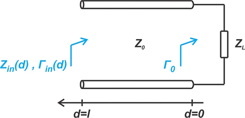
Figure 1. The transmission line terminated in an arbitrary impedance.
The input impedance of the transmission line at different points along the line is given through Equation 1:
\[Z_{in}(d) = Z_0\frac{1 + \Gamma_{in}(d)}{1-\Gamma_{in}(d)}\]
Equation 1.
Where Γin(d), the reflection coefficient at a distance, d, from the load, is shown in Equation 2:
\[\Gamma_{in}(d) = \Gamma_0 e^{-j2 \beta d}\]
Equation 2.
In Equation 2, β is the phase constant, and Γ0 is the familiar load reflection coefficient, which leads to Equation 3:
\[\Gamma_0 = \frac{Z_L - Z_0}{Z_L + Z_0}\]
Equation 3.
Equation 3 is easy to understand; it gives the load reflection coefficient for a given ZL. For example, if ZL = 50 + j50 Ω and Z0 = 50 Ω, we get Γ0 = 0.2 + j0.4. Equation 2 shows how the reflection coefficient changes along the line. As you can see, the magnitude of Γin(d) is constant and equal to the magnitude of Γ0 (0.447 with the above values); however, its phase angle varies linearly with distance from the load.
For example, if βd (known as the line’s electrical length) is 45°, the phase angle of Γin(d) is the phase of Γ0 minus 90° (63.4° - 90° = -26.6°). The following polar plot in Figure 2 shows how Γin(d) can be graphically obtained from Γ0.
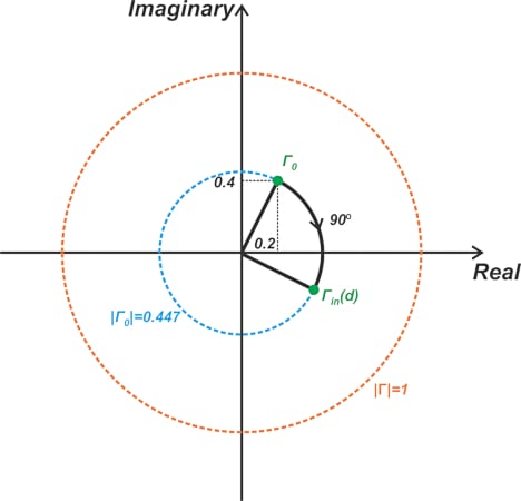
Figure 2. Example polar plot using the mentioned example and equations.
As can be seen, for a given Γ0, the reflection coefficient along the line Γin(d) lies on the circle having a radius of |Γ0|. To summarize, the reflection coefficient is a well-behaved RF parameter because its magnitude is constant along the line, and its phase angle changes linearly with the length of the line. This is not the case with the line’s impedance. With a mismatched load, the input impedance varies continuously along the line. For |Γ0| = 1, the magnitude of the input impedance can be anywhere between zero and infinity.
Reflection Coefficient for High-frequencies—Ease and Reliability of Measurements
There is another reason why the reflection coefficient is a more attractive parameter in high-frequency work. The concept of impedance naturally leads us to two-port network representations such as impedance parameters, admittance parameters, and hybrid parameters. To experimentally determine the parameters of these representations, we need to open-circuit or short-circuit the appropriate network port. At high frequencies, however, short- and open-circuit conditions are quite difficult to provide, especially over a broad frequency range. Furthermore, active high-frequency circuits may oscillate when terminated in open or short circuits.
On the other hand, the concept of the reflection coefficient is closely related to the S parameter representation. With this type of network representation, the appropriate port of the network is terminated in the characteristic impedance of the line. For example, the following diagram (Figure 3) measures two of the S parameters, namely S11 (the input reflection coefficient) and S21 (the transmission coefficient from port 1 to port 2).
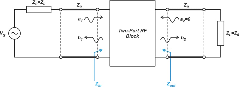
Figure 3. Example diagram showing two S parameters.
One major advantage of S parameters over other types of network representations is that broadband resistive terminations required for S parameter measurements are realizable in practice. This enables us to have accurate and repeatable RF measurements.
The Invention of the Smith Chart
Philip Smith, an AT&T engineer, invented the Smith chart in 1933 to simplify transmission lines’ input impedance calculations. As mentioned above, the Smith chart is a polar plot of the reflection coefficient. In those days, however, engineers were accustomed to working with the impedance concept; a graph of the reflection coefficient didn’t have much meaning to them.
First, we set a bit of context to realize the significance of Smith’s invention. The S parameters were introduced in the 1960s by K. Kurokawa. Network analyzers that use the S parameters to characterize the RF components into the gigahertz region were also introduced in the 1960s, more than 30 years after the invention of the Smith chart. Smith had recognized at least some of the advantages of the reflection coefficient over impedance and decided to use the Γ concept to solve the problems he was involved in. To be able to converse with other engineers in the familiar terms of the impedance parameter, Smith also decided to include some impedance plots so that one could easily find the equivalent impedance for a given reflection coefficient or vice versa. By plotting contours of constant resistance and reactance in the Γ-plane, the familiar Smith chart was created (Figure 4).
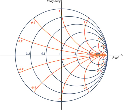
Figure 4. Example of a Smith chart.
In most Smith charts, the real and imaginary axis of the Γ-plane is not shown because there’s really no need to show them explicitly. This leaves us with some circles and arcs corresponding to the contours of constant resistance and reactance, respectively. Let’s see how these contours, which occasionally become intimidating and confusing, are obtained and how we can interpret them.
Smith Chart Normalized Impedance
The Smith chart is based on the relationship between Γ0 and impedance (Equation 3). It’s important to note that Equation 3 describes a one-to-one relationship between these two parameters, thereby knowing one is equivalent to knowing the other. Also, the Smith chart is plotted using the normalized impedance defined as follows:
\[z=\frac{Z_L}{Z_0}=r+jx\]
Equation 4.
Where r and x are the real and imaginary parts of the normalized impedance. Plotting the normalized impedance allows us to use the same chart for systems with different reference impedances. However, we need to keep in mind that the impedances we read from the chart should be multiplied by Z0 to find the actual impedance values for our system. Also, note that using a normalized impedance doesn’t change the Γ0 equation. To express Γ0 in terms of the normalized impedance, we divide both the numerator and denominator of Equation 3 by Z0, which obviously doesn’t change the equation. The Γ0 equation in terms of z is shown below:
\[\Gamma_0 = \frac{z-1}{z+1}\]
Equation 5.
Therefore, while the impedances shown on a Smith chart are normalized, the reflection coefficient is not. Equation 5 is the mapping function determining how a given z produces its corresponding Γ. This equation is actually a bilinear transformation. The name stems from the fact that it is the ratio of two linear functions. Bilinear transformations map circles into circles. Remember that for mathematicians, straight lines are also special cases of circles.
Constant Resistance Circles
Being a bilinear transformation, Equation 5 maps the lines of constant r (or impedances with a constant real part) to a circle in the Γ-plane. For example, the line z = 0 + jx is transformed to a circle of radius 1 centered at the origin of the Γ-plane (see the blue line and blue circle below in Figure 5).
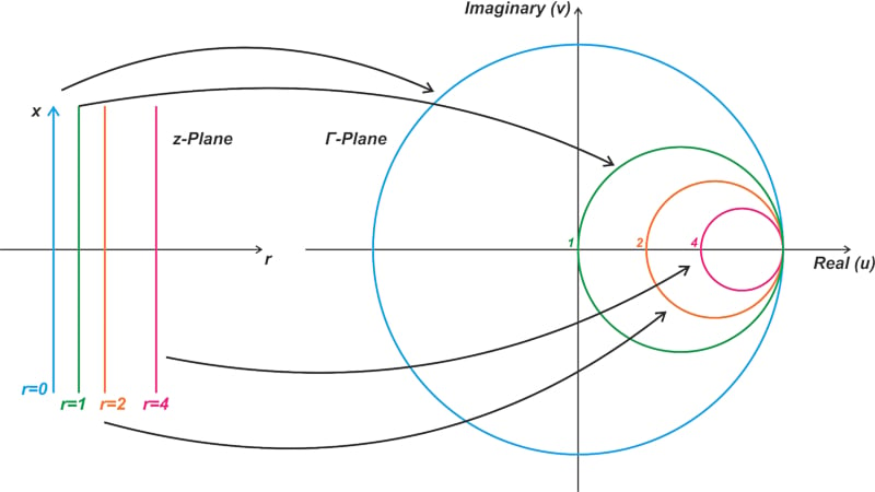
Figure 5. Example bilinear transformation.
Similarly, the transformation maps the line z = 1 + jx to a circle of radius 0.5 centered at u = 0.5 and v = 0. In general, it can be shown that impedances with constant r are transformed to a circle of radius \(\frac{1}{r+1}\) centered at \(u = \frac{r}{r+1}\) and v = 0.
Constant Reactance Circles
The mapping of impedances with a constant reactance for some values of x is shown in Figure 6.
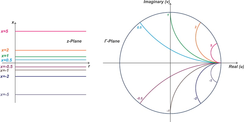
Figure 6. Example mapping of impedances with a constant reactance.
Again, the bilinear transformation of Equation 5 maps lines of constant x (or impedances with a constant imaginary part) to a circle in the Γ-plane. Note that only the portion of these circles that lies inside the unit circle is shown in the above figure. When working with passive loads, |Γ| cannot exceed unity. This means that impedances have an r ≥ 0 map inside the unit circle. That’s why we’re usually interested in the region confined to the unit circle when working the Smith chart. Only a portion of the constant reactance circles falls inside the unit circle, and therefore, these curves appear as some arcs rather than complete circles.
In general, impedances with constant x are transformed to a circle of radius \(\frac{1}{x}\) centered at u = 1 and \(v=\frac{1}{x}\). The Smith Chart is a polar plot of the reflection coefficient overlaid with the above constant resistance and reactance contours (Figure 4 above).
In the next article, we’ll look at several different examples of impedance calculations by means of the Smith chart
To see a complete list of my articles, please visit this page.
Related Content