 Facebook
 Google
 GitHub
 Linkedin
Exploring Single Stub Impedance Matching Through Smith Chart Examples
Learn about impedance matching using a single stub, transmission lines, and immittance Smith chart examples.
Since inductors and capacitors can be very lossy at high frequencies, we normally prefer to use a transmission line-based impedance-matching network in high-frequency applications. The basic concepts of this technique, along with an introductory example, were presented in the previous article. The Smith chart was an invention of the electrical engineer Phillip Hagar Smith.
In this article, we’ll expand our knowledge through several different examples of applying this technique.
Impedance Matching Via a Single Transmission Line
We know that a transmission line section produces a motion along a constant |Γ| circle on the Smith chart. It is sometimes possible to provide a match by only adjusting the length of the line. As an example, consider the following diagram shown in Figure 1.
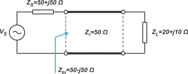
Figure 1. Example transmission line diagram.
Assume that we need to transform the load impedance ZL = 20 + j10 Ω to the complex conjugate of the source impedance ZS = 50 + j50 Ω—to provide a complex conjugate match between the load and source. With a normalizing impedance of Z0 = 50 Ω, we locate the normalized impedances zL and zS on the Smith chart (Figure 2).

Figure 2. Smoth chart showing a normalized impedance [click image to enlarge].
The figure shows that both zS and zL lie on the |Γ| = 0.447 circle. This allows us to use a single transmission line element as the impedance-matching network. The complex conjugate of zS is marked as point A on the Smith chart. On the wavelength scale, points zL and A correspond to 0.037λ and 0.338λ; therefore, a line of length 0.338λ - 0.037λ = 0.301λ can do the job.
Stub Matching—Four Arrangements for Adding a Single Stub
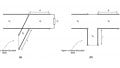
The load and source impedances are most often on different |Γ| circles. In these cases, we can add a parallel transmission line element, known as a stub, to an appropriate point of the series line to provide a match. With a single stub, there are four different possible arrangements (Figure 3).
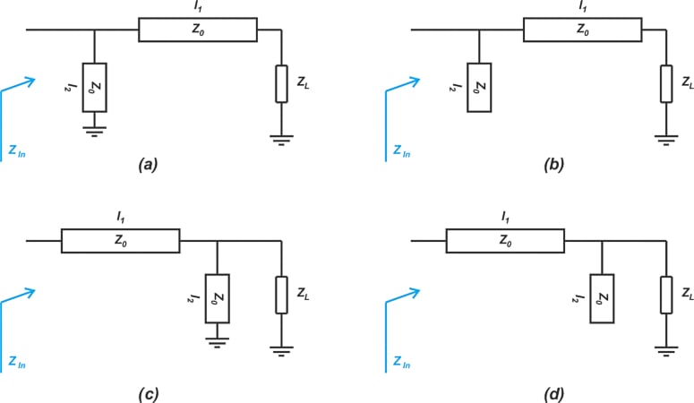
Figure 3. Different arrangements of four different single stubs.
In Figures 3(a) and (b), the series line (also sometimes referred to as the cascade line) is used first, whereas Figures 3(c) and (d) start with a stub at the load end. Whether a series line or a parallel stub is connected to a given termination depends on the value of ZL and ZIn. Also, note that the stubs in Figures 3(a) and (c) are short-circuited, while those in (b) and (d) terminate in an open-circuited load. With a properly selected combination of a series line and a parallel stub, we can transform an arbitrary impedance to another desired value.
Before diving in too far, note that, with these matching networks, the series line and the stub element normally have identical characteristic impedance Z0. This choice is made to avoid unnecessarily complicating the design task. Using identical characteristic impedances, we’re left with two unknown parameters: the length of the series line (l1) and the length of the stub (l2).
Example 1: From the Center of the Smith Chart to an Arbitrary Point
Using an immittance Smith chart, design a matching network to transform ZL = 50 Ω to ZIn = 50 + j100 Ω.
With a normalizing impedance of Z0 = 50 Ω, we locate the normalized load and target impedance (zL = 1, zIn = 1 + j2) on the immittance Smith chart (Figure 4).

Figure 4. Immittance Smith chart showing a normalized load and target impedance [click image to enlarge].
A stub element acts like a parallel capacitor or a parallel inductor at the frequency of interest, producing a motion along a constant-conductance circle. Therefore, working with a series line and a parallel stub, we should use the constant-conductance circle going through one point with the constant |Γ| circle that goes through the other point. In this example, zL is at the center of the Smith chart, and we’re left with only one option for this point: the constant-conductance circle going through zL, which is the g = 1 circle. This circle intersects the |Γ| = 0.71 circle going through zIn at points A and B, as shown in the above figure. Therefore, we have two different solutions. The path going through point A is shown below in Figure 5.

Figure 5. Smith chart showing a path that goes through point A [click image to enlarge].
Since the first motion is along a constant-conductance circle, the parallel stub should be at the load end (Figure 3(c) or (d)). Also, the parallel stub should produce a susceptance equal to that of the intersection point (point A), which is -j2 in this example. As shown in Figure 6, a short-circuited stub of length l2 = 0.074λ or an open-circuited stub of length l2 = 0.324λ can produce the required susceptance. This moves us from zL to point A.

Figure 6. Smith chart showing the shift from zL to point A [click image to enlarge].
Here, we choose a short-circuited stub to have the shortest possible length. Finally, we use a series line of length l1 = 0.125λ to produce the circular motion from point A to zIn (Figure 7).
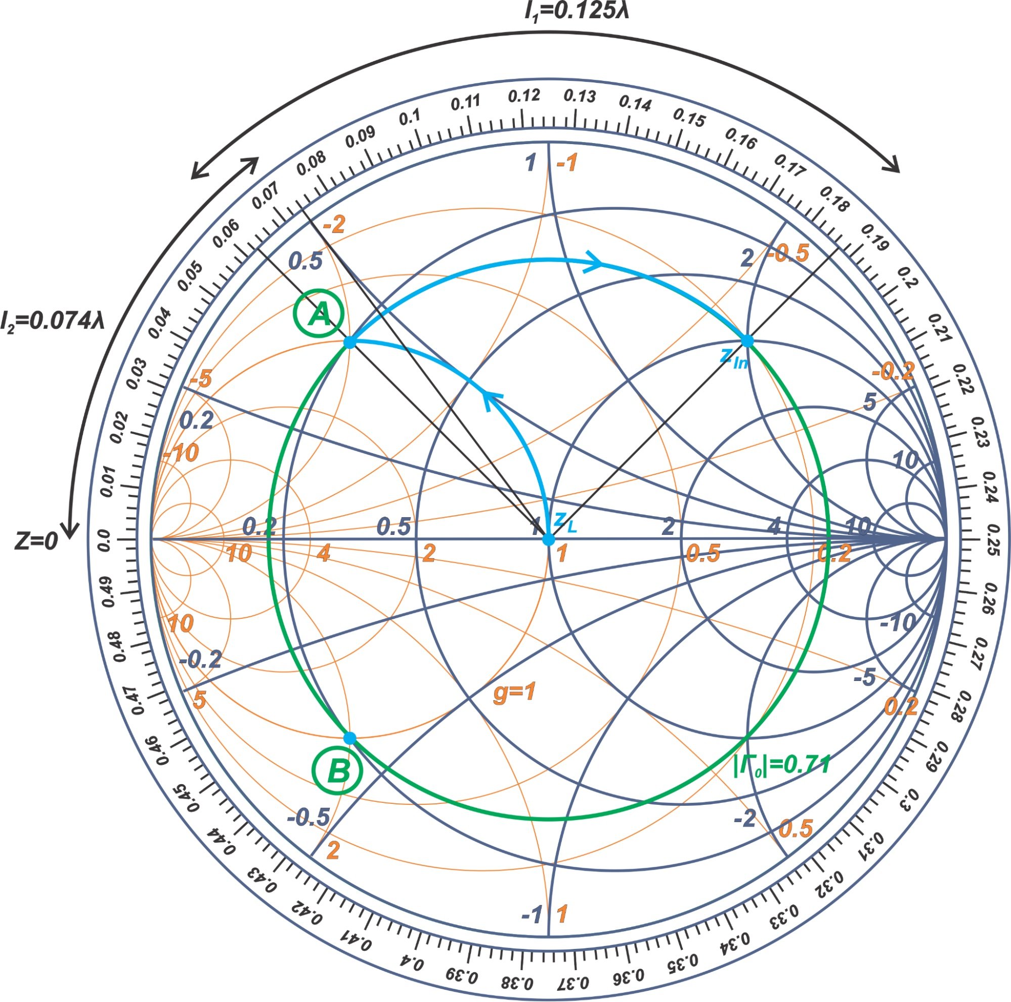
Figure 7. Smith chart showing the circular motion from point A to zIn [click image to enlarge].
The final matching circuit is shown in Figure 8.
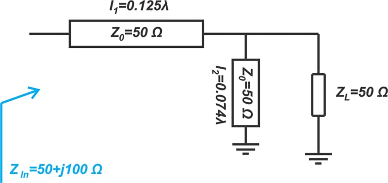
Figure 8. Final matching circuit for the above example.
Similarly, we could use the path going through point B to design the matching network. In this case, the length of the open-circuited stub and the series line is found to be l2 = 0.176λ and l1 = 0.25λ, as shown below in Figure 9.
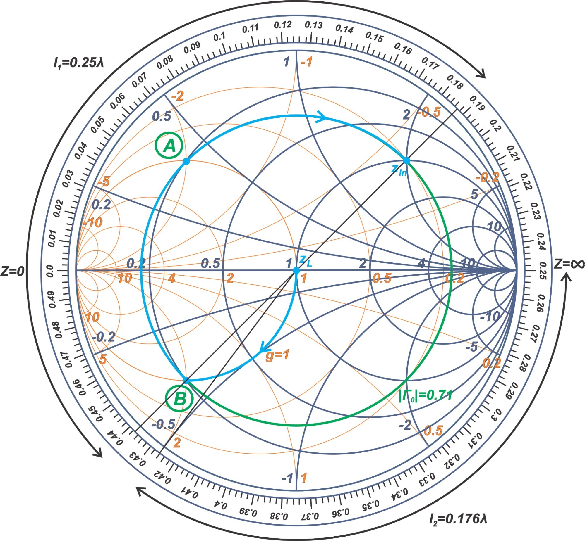
Figure 9. Smith chart showing the length of the open-circuited stub and series line at l2 = 0.176λ and l1 = 0.25λ [click image to enlarge].
Figure 10 shows the matching circuit.
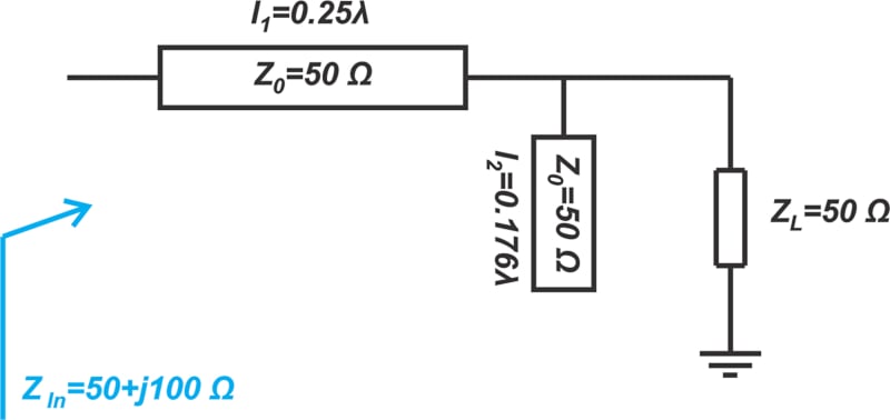
Figure 10. Matching circuit for Figure 9.
Example 2: From an Arbitrary Point to the Center of the Smith Chart
Using an immittance Smith chart, design a matching network to transform ZL = 100 + j100 Ω to ZIn = 50 Ω.
With a normalizing impedance of Z0 = 50 Ω, we locate the normalized load and target impedance (zL = 2 + j2, zIn = 1) on the immittance Smith chart (Figure 11).
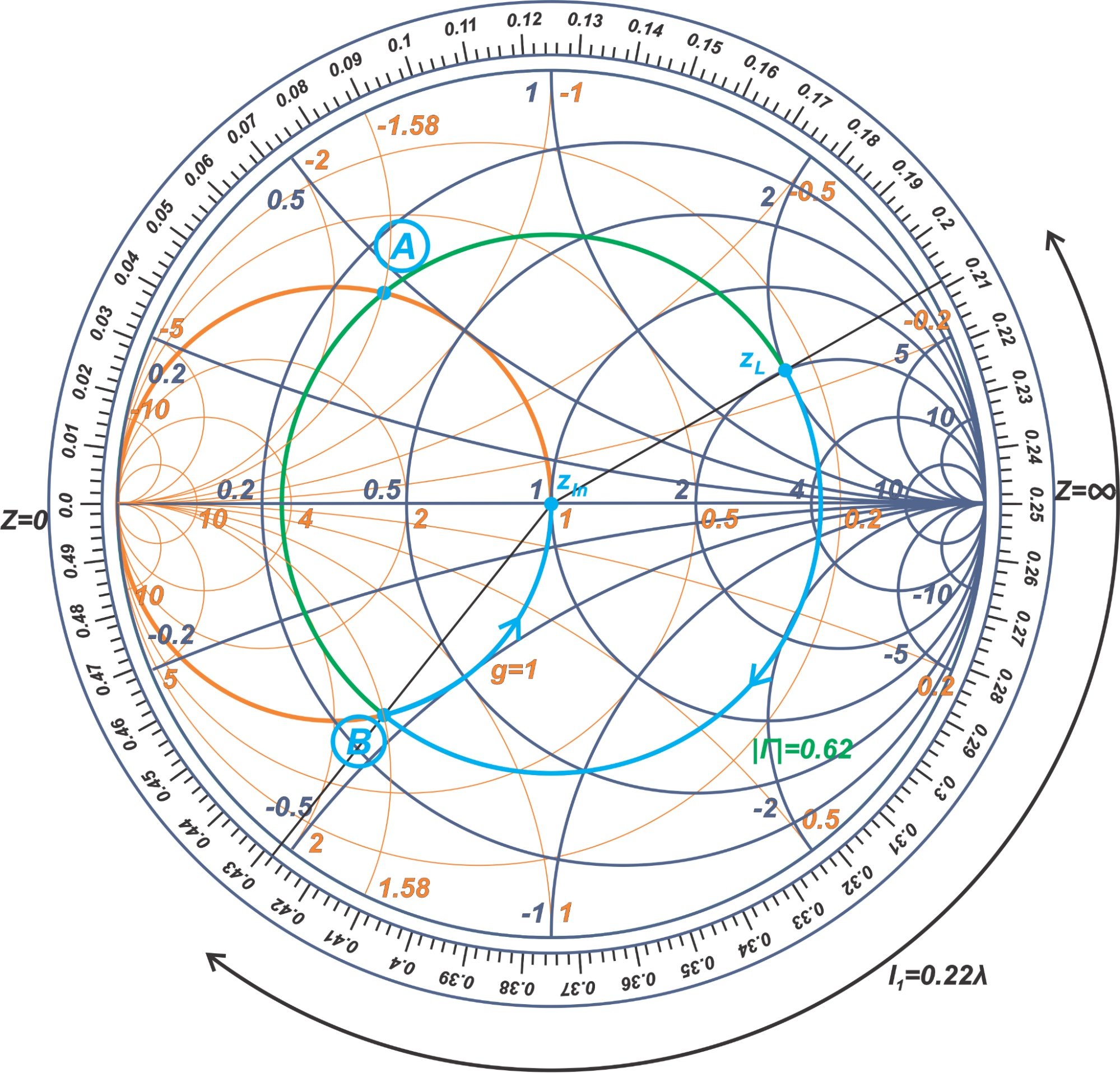
Figure 11. Immittance Smith chart showing the normalizing impedance to locate the normalized load and target impedance [click image to enlarge].
To go from an arbitrary load to the center of the Smith chart, we should first use a constant |Γ| circle to move to a point on the g = 1 constant-conductance circle. As shown in the above figure, the constant |Γ| circle going through zL (the |Γ| = 0.62 circle) intersects the g=1 circle at two points (points A and B). To have the shortest possible line, we choose point B. The cyan path in the figure shows the motion that takes us from zL to point B and then to the center of the Smith chart. The motion from point B to the center of the chart requires a shunt stub. Therefore, the configurations in Figures 3(a) and (b) work for this problem. The length of the series line is found by measuring the corresponding arc on the wavelength scale that works out to l1 = 0.22λ, as shown in the above figure.
To find the length of the stub l2, we need to know the susceptance of point B. Using a more detailed Smith chart, you can verify that the admittance value at point B is yB = 1 + j1.58. Let’s assume that we are going to use a short-circuited stub (this actually leads to a shorter length stub). The circuit diagram we have obtained so far is shown below (Figure 12).
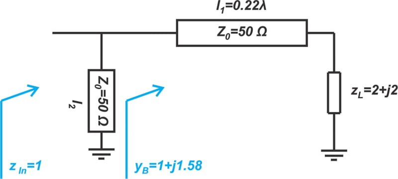
Figure 12. Circuit diagram with the information we've found so far in our example.
We need the stub to provide a normalized susceptance of -j1.58 to cancel out the susceptance of point B and move us to the center of the Smith chart. In Figure 13, the length of the short-circuited stub works out to l2 = 0.09λ.

Figure 13. Smith chart with a short-circuited stub of l2 = 0.09λ [click image to enlarge].
If you compare Examples 1 and 2, you’ll notice an important difference in their design procedure. In Example 1, the parallel stub produced a susceptance value equal to that of the intersection point. However, in Example 2, the parallel stub produced a susceptance equal to the negative of the susceptance of the intersection point to cancel it out and move us to the center of the Smith chart. When designing transmission line-based impedance matching networks, one needs to analyze the problem carefully to choose the right susceptance value for the problem at hand.
Interpreting a Z Smith Chart as a Y Smith Chart
It is possible to perform the above calculations using only an impedance Smith chart. Many references use this method, so our final example below will use a Z Smith chart. With this method, we actually interpret the Z Smith chart as an admittance (or Y) Smith chart. This interpretation is based on the idea that a Y Smith chart can be obtained by rotating the Z Smith chart by 180°. In order to use a Z Smith chart for admittance manipulations, we interpret constant-resistance (r) circles as constant-conductance (g) circles; and constant-reactance (x) circles as constant-susceptance (b) circles. Be careful, as the capacitors are now at the top of the chart, and the inductors are at the bottom. The short and open circuit points likewise swap positions. When we use a Z Smith chart as a Y Smith chart, we are effectively rotating our own position (or our angle of observation) by 180° with respect to the chart (i.e. instead of rotating the chart by 180°, we rotate our angle of observation). If necessary, we can interpret the chart as either an impedance Smith chart or an admittance Smith chart at different stages of the solution.
One final note before we look at the example: when designing impedance matching networks by means of a Z Smith chart, we usually need to convert an impedance to its equivalent admittance. To find the admittance corresponding to a given zL, we locate zL on the chart and rotate by 180° on the corresponding constant |Γ| circle. Now, we read off the impedance value from the chart. This value is equal to the admittance of zL.
Example 3: Design a Matching Network Using an Impedance Smith Chart
Using an impedance Smith chart, design a matching network to transform ZL = 100 + j100 Ω to ZIn = 50 Ω.
We first locate the normalized impedance zL = 2 + j2 on the Smith chart (Figure 14).

Figure 14. Smith chart showing the normalized impedance of zL = 2 + j2 [click image to enlarge].
Rotating by 180° along the constant |Γ| circle, we move from zL to point B. The impedance value of this point is actually equal to the admittance of zL. Therefore, from the above chart, the normalized admittance of the load is yL = 0.25 - j0.25.
Now, interpreting the chart as an admittance chart, we follow the constant |Γ| circle in a clockwise direction to move to the g = 1 circle. This point is marked as point C in the chart. As shown in the figure, this rotation corresponds to a series line of length l1 = 0.22λ.
At point C, the normalized admittance is yC = 1 + j1.58. Therefore, the shunt stub should produce a susceptance of -j1.58 to move us to the center of the chart. This can be achieved by a short-circuited stub of length l2 = 0.09λ, as shown in the above figure. Note that when interpreting the Z Smith chart as a Y Smith chart, the short and open circuit points swap positions. The final matching circuit is shown in Figure 15.
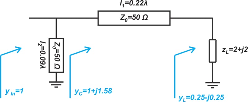
Figure 15. The final matching circuit diagram for Example 2.
Note that, in this example, we solved the impedance matching problem of Example 2 using a Z Smith chart. As you can see, the results of these two methods (Figure 15 and Figure 12) are the same.
Single Snub and Impedance Matching Summary
With a properly selected combination of a series line and a parallel stub, we can transform an arbitrary impedance to another desired value. Design of these matching networks can be easily done through an immittance Smith chart. Another option is to use a Z Smith chart as a Y Smith chart. The design of impedance matching networks using a Smith chart is fast, intuitive, and usually accurate enough in practice.
To see a complete list of my articles, please visit this page.


When developing the Smith chart, there are certain precautions that should be noted. These are among the most important:
All the circles have one same, unique intersecting point at the coordinate (1, 0).
The zero Ω circle where there is no resistance (r = 0) is the largest one.
The infinite resistor circle is reduced to one point at (1, 0).
There should be no negative resistance. If one (or more) should occur, we will be faced with the possibility of oscillatory conditions.
Another resistance value can be chosen by simply selecting another circle corresponding to the new value.