Facebook
 Google
 GitHub
 Linkedin
Design a Two-element Matching Network Using the ZY Smith Chart
Learn about the immittance Smith chart (ZY Smith chart), the effect of adding series and parallel components, impedance matching, and finding a two-element matching network.
Previously in this series, we discussed how series and parallel circuits can be conveniently analyzed using impedance Smith charts and admittance Smith charts, respectively. When dealing with both parallel and series components, we can use a chart that includes both the impedance and admittance plots. The Smith chart with both the impedance and admittance contours is known as the immittance Smith chart (or the ZY Smith chart). The Smith chart was an invention of the electrical engineer Phillip Hagar Smith.
The ZY Smith Chart
The immittance Smith chart is shown in Figure 1.
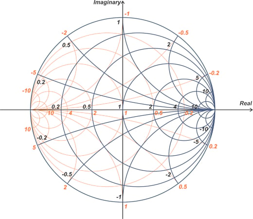
Figure 1. Example immittance Smith chart.
With an immittance Smith chart, we can easily find the equivalent admittance of a given impedance or vice versa. For example, assume that the normalized load impedance is z1 = 1 + j1. We can locate z1 in the immittance Smith chart and directly read from the orange curves its equivalent admittance. This is illustrated below in Figure 2.
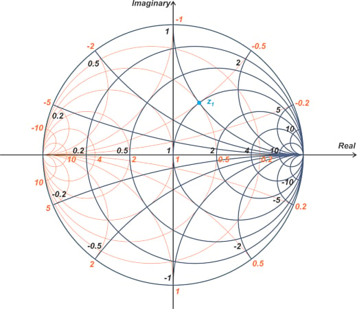
Figure 2. Using an immittance Smith chart's orange curves to find the equivalent admittance of z1.
From the above chart, we find the equivalent admittance y1 = 0.5 - j0.5. When using the immittance chart, there is one main caveat: be careful to use the correct numbers for the curve you’re working with. To avoid such errors, keep in mind that circles (or arcs) larger than the r = 1 circle (or the x = 1 arc) correspond to smaller numbers. For example, in the above graph, one might doubt whether the conductance value of the orange circle going through z1 is 2 or 0.5. However, since this circle is larger than the r = 1 circle, we know that its associated value is the smaller one (0.5).
Effect of Adding Parallel and Series Components
The following figure (Figure 3) shows how adding reactive components change our position on the immittance chart.
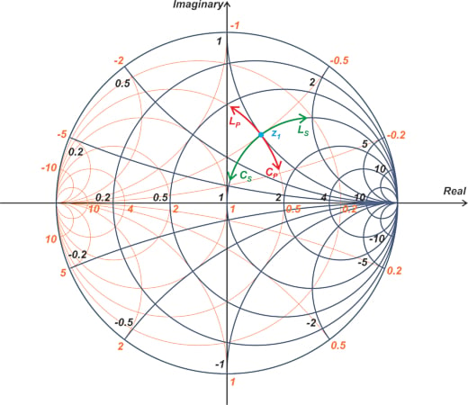
Figure 3. An immittance Smith chart with reactive components.
When adding a series reactive component, the real part of the impedance is constant, and thus, the overall impedance moves along the constant-resistance circle. If a series inductor, LS, is added, the impedance moves in a clockwise direction. On the other hand, with a series capacitor, CS, the motion is in a counterclockwise direction.
Adding a parallel reactive component moves us on a constant-conductance circle. If a parallel inductor, LP, is added, the admittance moves in a counterclockwise direction. For a parallel capacitor, CP, the motion is in a clockwise direction. Figure 4 shows how adding a series resistor, RS, or a parallel resistor, RP, moves us on a constant-reactance or constant-susceptance arc, respectively.
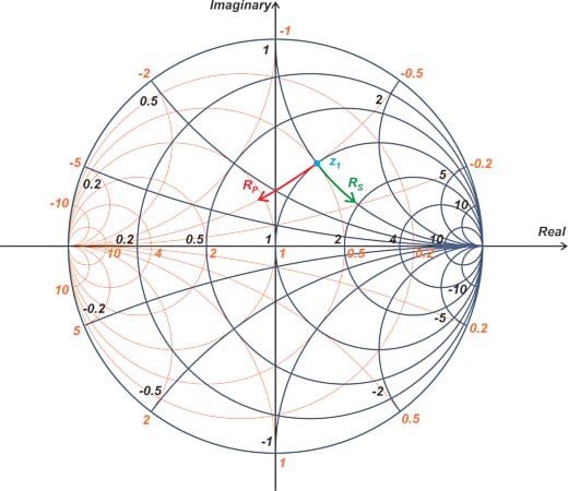
Figure 4. Immittance Smith chart shows how adding a series or parallel resistor moves the constant-reactance or constant-susceptance arc, respectively.
One important application of the Smith chart is the design of impedance-matching networks, which will be discussed in the rest of the article.
Impedance Matching—Transforming One Impedance to Another
Impedance transformation or matching is a major concern in RF design, so much so that some engineers state that RF design is all about impedance matching. The need for impedance matching arises for various reasons. For example, in order to reduce electrical wave reflections, we need to match the load impedance to the line’s characteristic impedance.
Finding the Appropriate Two-element Matching Network
Using the immittance Smith chart, we can easily find two-element lossless matching networks. Let’s examine this through an example. Assume that the load impedance Z1 = 10 + j10 Ω is to be matched to a source impedance of Z2 = 50 Ω. With a normalizing impedance of Z0 = 50 Ω, the normalized impedances are z1 = 0.2 + j0.2 and z2 = 1 (Figure 5).
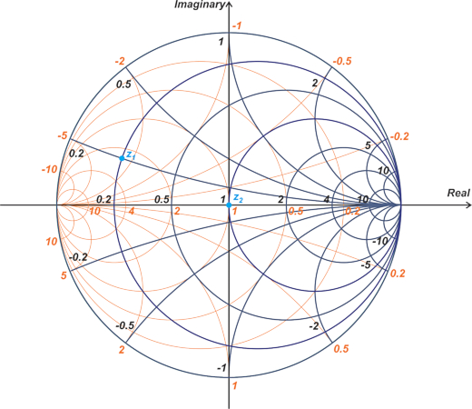
Figure 5. An immittance Smith chart showing the normalizing impedances.
We aim to find two-element lossless matching networks that transform z1 to z2. Since we’re designing a lossless matching network, we cannot add resistors. We can only add parallel or series reactive components. As a result, the design of the matching network involves moving along either constant-resistance or constant-conductance circles that pass through points z1 and z2. Figure 6 shows these circles with the other circles and arcs removed for clarity.
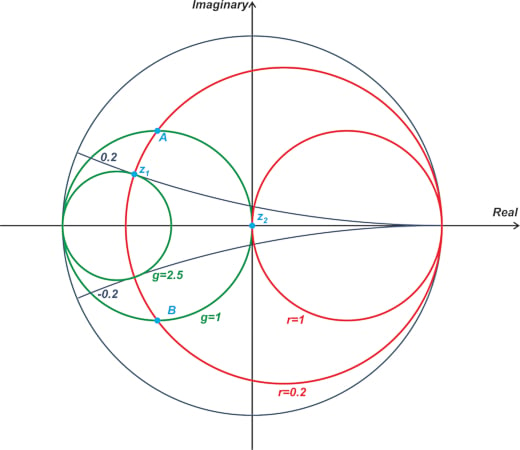
Figure 6. Example chart showing the constant-resistance or constant-conductance circles for a matching network.
Since there are two different circles that go through z1 and z2, in order to move from z1 to z2, we need to use one circle passing through z1 with another one going through z2. Clearly, these two circles should intersect each other. In the above example, the r = 0.2 constant-resistance circle that goes through z1 and the g = 1 constant-conductance circle that passes through z2 meet these conditions. These two circles intersect at points A and B; therefore, we can have two different paths from z1 to z2. The cyan and orange paths below show these two possible options (Figure 7).
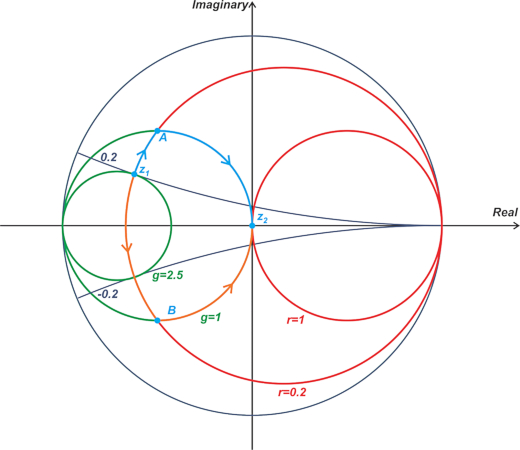
Figure 7. Chart showing the intersecting points A and B.
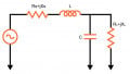
The motion from z1 to point A corresponds to a series inductor, while the motion from A to z2 is produced by a parallel capacitor. Therefore, the two-element arrangement shown below can be used to transform z1 to z2.
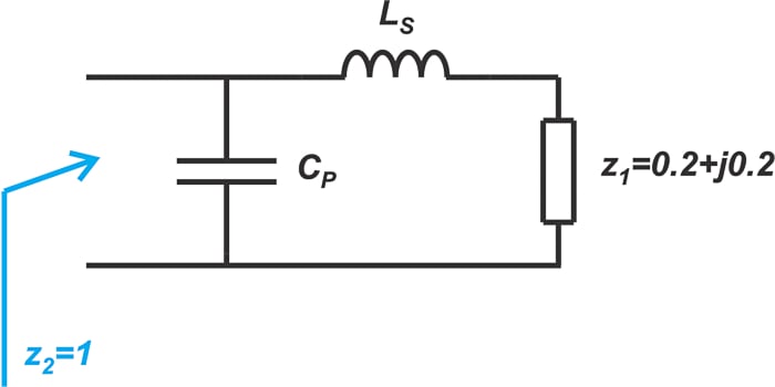
Figure 8. Example two-element arrangement.
The orange path in Figure 7 corresponds to a series capacitor (from z1 to B) and a parallel inductor (from B to z2). This gives us another matching network, as shown in Figure 9.
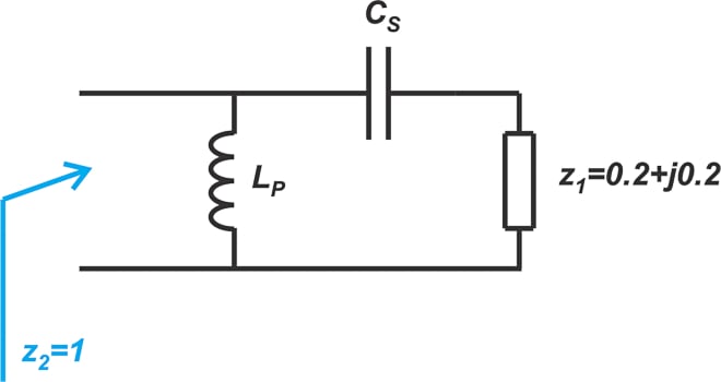
Figure 9. A matching network diagram.
Finding Matching Network Component Values
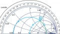
To find the component values of the above matching networks, we need to know the reactance and susceptance of points A and B. With a commercial Smith chart, there is a sufficient number of impedance and admittance contours to estimate the values associated with an arbitrary point on the chart with reasonable accuracy. The Smith chart in Figure 10 shows the reactance and susceptance values of points A and B.
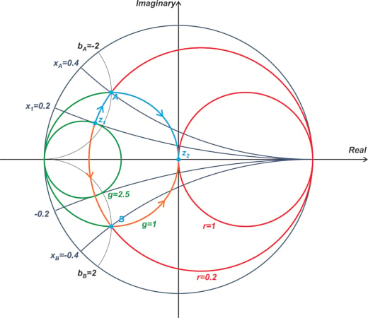
Figure 10. Smith chart showing the reactance and susceptance values of points A and B.
To move from z1 to A, the series inductor should have a normalized reactance of xA - x1 = j0.2. Assuming that the frequency of operation is 1 GHz, we have:
\[\frac{L_s \omega}{Z_0}=0.2 \Rightarrow L_s=\frac{0.2 \times 50}{2 \pi \times 1 \times 10^{9}}=1.59 \text{ } nH\]
To go from point A to z2, we need a parallel capacitor with normalized susceptance of j2. This, in turn, zeros out the initial susceptance we have at point A and moves us to the origin of the Smith chart. The capacitor value at 1 GHz is found as:
\[\frac{C_p \omega}{Y_0}=2 \Rightarrow C_p=\frac{2 \times 0.02}{2 \pi \times 1 \times 10^{9}}=6.37 \text{ } pF\]
The final matching network obtained from the cyan path is shown in Figure 11.
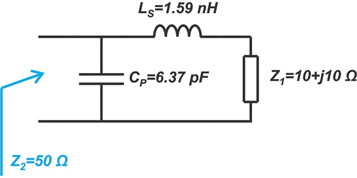
Figure 11. Matching network diagram from the cyan path in the Smith chart we've been using throughout this article.
If you calculate the input impedance of the above circuit, you’ll find zin = 49.96 - j0.03 Ω, which is reasonably close to the target 50 Ω impedance. Similarly, we can find the component values for the circuit in Figure 9. In this case, a series capacitor with a normalized reactance of xB - x1 = -0.4j - 0.2j = -0.6j is needed to move from point z1 to B. At 1 GHz, the capacitor value is:
\[\frac{1}{C_s \omega Z_0}=0.6 \Rightarrow C_s=\frac{1}{0.6 \times 2 \pi \times 1 \times 10^{9} \times 50}=5.31 \text{ } pF\]
Next, a parallel inductor with a normalized susceptance of -2 is needed to move from point B to the origin of the Smith chart. The inductor value is:
\[\frac{1}{L_p \omega Y_0}=2 \Rightarrow L_p=\frac{1}{2 \times 2 \pi \times 1 \times 10^{9} \times 0.02}=3.98 \text{ } nH\]
Using these values, the final matching network is obtained, as shown in Figure 12.

Figure 12. A final matching network diagram.
Again we can find the input impedance to verify our calculations. The input impedance of the above circuit is 49.89 - j0.11 Ω which is close to the desired value. The matching networks we found above are called L-sections or L-networks. The term “L” is used because the two lumped elements form the letter L in the circuit diagram. By combining two reactive components, we can have a total of eight different L-section matching networks. In the following section, we’ll take a brief look at some other L-sections.
Four Different L-sections for One Impedance Matching Problem
In the example depicted in Figure 10, only two of the circles crossed each other. As another example, consider transforming the impedance, z3, shown in Figure 13, to the origin of the Smith chart.
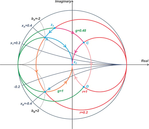
Figure 13. Chart showing the transformation of impedance z3.
This example has some similarities to the previous one. In fact, three of the circles in these two examples are the same (the r = 1, r = 0.2, and g = 1 circles are the same). The initial impedance, z3, is only moved a little bit upward so that its constant-conductance circle (g = 0.48) intersects the constant-resistance circle of the target impedance (r = 1). This produces two new intersection points (points C and D). Due to this change, two new impedance matching options are available. The four different L-sections that can be used for this problem are shown in Figure 14.
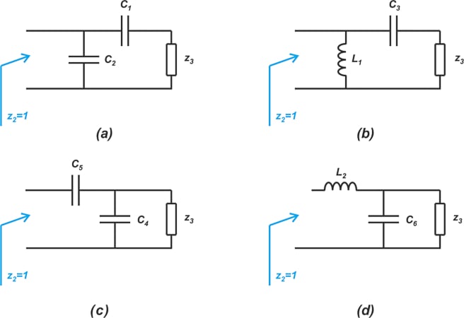
Figure 14. Four different L-section diagrams.
The L-sections in Figure 14 (a), (b), (c), and (d) correspond to paths going through the intersection points A, B, C, and D, respectively. As can be seen, for a given matching problem, we might have either two or four different L-type matching solutions. When choosing the appropriate matching network, there are several different considerations. Bandwidth, frequency response, and ease of implementation are three of important factors that should be considered. In the next article, we’ll dive deeper into this topic.
To see a complete list of my articles, please visit this page.
Related Content