Facebook
 Google
 GitHub
 Linkedin
Analyze RLC Components Using the Admittance Smith Chart and Examples
Learn about the admittance Smith chart to analyze a parallel connection of resistors, capacitors, and inductors, and see the circuit's behavior over the swept frequency range.
Since network analyzers display the reflection coefficient data versus frequency directly on a Smith chart, it’s important to be familiar enough with the Smith chart to easily recognize what combination of RLC components can produce the displayed contour. In a previous article, we used an impedance Smith chart to examine the frequency response of series RC, RL, and RLC circuits. The Smith chart was an invention of the electrical engineer Phillip Hagar Smith.
In this article, we’ll derive the admittance Smith chart that allows us to easily analyze a parallel connection of resistors, capacitors, and inductors. We’ll see that by sweeping the frequency, the admittance of the parallel circuit produces a contour on the Smith chart that describes the circuit behavior over the swept frequency range.
Developing the Admittance Smith Chart
The frequency response of series RC, RL, and RLC circuits can be easily analyzed by means of an impedance Smith chart. From circuit theory concepts, we know that when dealing with parallel connections of RLC components, the use of the admittance (Y) concept can simplify the calculations. In a similar manner, we can develop a plot of the admittance contours in the Γ-plane to analyze the parallel connection of components. This gives us a new Smith chart known as the admittance Smith chart.
Let’s see how we can use our knowledge of the impedance Smith chart to derive the admittance Smith chart. The impedance Smith chart is actually a plot of the following mapping function for some specific values of z in the Γ-plane:
\[\Gamma = \frac{z-1}{z+1}\]
Equation 1.
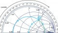
Here z = r + jx is the normalized impedance. A plot of the above mapping function for some constant values of resistance, r, and reactance, x, gives us an impedance Smith chart, as shown below in Figure 1.
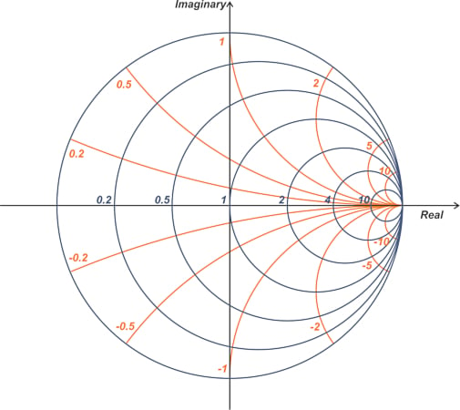
Figure 1. Example impedance Smith chart.
As electronics engineers, we know the physical interpretation of the parameter z in Equation 1 represents the impedance of a circuit. However, from a mathematical point of view, z is only a complex number and can represent any complex parameter. In other words, having the impedance Smith chart, we know how Equation 1 maps an arbitrary complex number z into the Γ-plane. In order to use this knowledge to derive the admittance contours in the Γ-plane, we only need to write the relationship between Γ and admittance Y in the form of Equation 1. The reflection coefficient equation in terms of impedance is:
\[\Gamma = \frac{Z - Z_0}{Z + Z_0}\]
Substituting \(Z=\frac{1}{Y}\) and \(Z_{0}=\frac{1}{Y_{0}}\), where Y0 is the reference admittance, we get:
\[\Gamma = \frac{Y_0 - Y}{Y_0 + Y}\]
Dividing both the numerator and denominator by Y0 and defining the normalized admittance \(y=\frac{Y}{Y_{0}}\), gives us Equation 2.
\[\Gamma =- \frac{y-1}{y+1}\]
Equation 2.
Noting that y is a complex number (y = g + jb), the mapping function in Equation 2 is the same as that in Equation 1, except that it is multiplied by -1. Due to this algebraic change, the admittance contours in the Γ-plane are obtained by rotating the impedance Smith chart by 180° (because -1 = ejπ). An admittance Smith chart is shown in Figure 2.
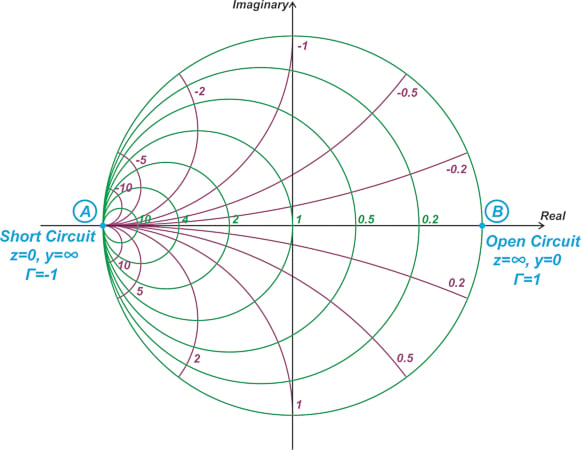
Figure 2. Example of an admittance Smith chart.
Admittance Smith Chart Key Points
The admittance Smith chart provides a plot of the normalized admittance y = g + jb in the Γ-plane, where g and b, respectively, represent the conductance and susceptance of y. Note that, due to the 180° rotation discussed above, the upper half of the chart corresponds to negative values of b (or negative susceptances). This makes sense because we know that inductive impedances appear at the upper half of the impedance Smith chart, and an inductive load also has a negative susceptance b. On the other hand, the lower part of the admittance Smith chart corresponds to positive susceptances (or capacitive components).
The admittance Smith chart in Figure 2 also shows the location of short-circuited (z = 0, y = ∞, Γ = -1) and open-circuited (z = ∞, y = 0, Γ = 1) loads. Note that the location of the short circuit and open circuit loads are consistent with those of the impedance Smith chart. This should be no surprise because we have only plotted some admittance contours in the Γ-plane, which obviously doesn’t change the location of the short and open circuit loads.
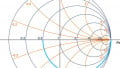
The circles in the above chart correspond to lines of constant conductance, g, in the y-plane (see Figure 3).
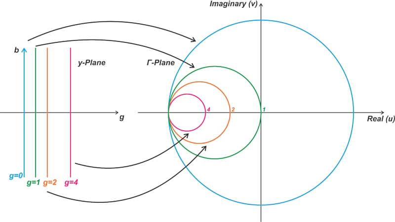
Figure 3. Smith chart circles corresponding to the lines of constant conductance in the y-plane.
Note that for passive loads, |Γ| cannot exceed unity, and we’re dealing with admittances having a positive conductance, g ≥ 0. Also, as shown in Figure 4, the arcs in the admittance Smith chart correspond to lines of constant susceptance.
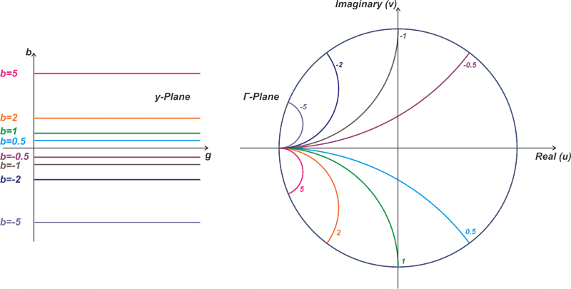
Figure 4. Visual of the arc in the admittance Smith chart corresponding with the lines of constant susceptance.
As you can see, the smaller circles and arcs correspond to larger values of conductance and susceptance, respectively. Therefore, if you increase the g or b component of the admittance, you’ll move toward smaller circles and arcs in the Smith chart.
At a given frequency, a parallel RLC circuit has an equivalent normalized admittance y = g + jb and, therefore, can be represented by a point on the admittance Smith chart. If the frequency is swept, the imaginary part of the admittance changes, and we obtain an admittance contour on the Smith chart that describes the circuit's behavior. Let’s look at some examples.
Admittance Smith Chart Examples
In this section, you'll find six different examples that help build on various admittance smith chart concepts as we go along.
Example 1: Adding a Parallel Capacitor
With a normalized load admittance of y1 = 0.2 - j0.5, the reflection coefficient is Γ1 = 0.72 $$\angle$$ 54.62° (Equation 2). If we add to this admittance a 10 pF parallel capacitor (C1 = 10 pF), what would be the new admittance and reflection coefficient?
Assume that the operating frequency is 222.82 MHz and the reference admittance is Y0 = 20 mS (that corresponds to a reference impedance of Z0 = 50Ω).The load admittance y1 and the associated reflection coefficient Γ1 are shown in Figure 5.
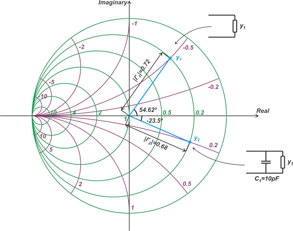
Figure 5. Admittance Smith chart showing the load admittance (y1) and the associated reflection coefficient (Γ1).
The parallel capacitor affects only the susceptance of the new admittance. Therefore, the new admittance also lies on the g = 0.2 constant-conductance circle. At 222.82 MHz, a 10 pF capacitor has a normalized susceptance of j0.7:
\[\begin{eqnarray}
jb &=& \frac{j2 \pi f C}{Y_0} \\
&=& \frac{j2 \pi \times 222.82 \times 10^6 \times 10 \times 10^{-12}}{0.02}=j0.7
\end{eqnarray}\]
The capacitor increases the initial susceptance by j0.7, moving us from the -j0.5 to j0.2 constant-susceptance arc. The new admittance, y2, is at the intersection of the g = 0.2 constant-conductance circle and the b = 0.2 constant-susceptance arc, as shown in the above figure. Measuring the length and phase angle of the vector from the origin to y2, we obtain Γ2 = 0.68 $$\angle$$ -23.5°.
If we add a second 10 pF parallel capacitor (C2 = 10 pF) to y2, what would be the new admittance y3? The new capacitor increases the susceptance by another j0.7. Therefore, we end up at point y3 = 0.2 + j0.9, as shown below (Figure 6).
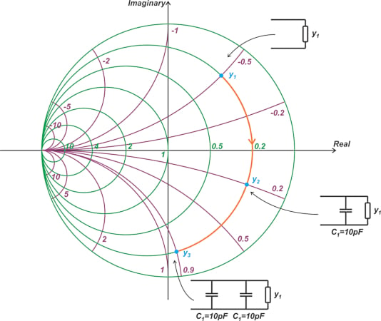
Figure 6. An admittance Smith chart shows that continuing to add more parallel capacitors moves the admittance clockwise along the constant-conductance circle.
The above example shows that by continuing to add more and more parallel capacitors, the overall admittance moves along the constant-conductance circle in a clockwise direction.
Example 2: Sweeping the Value of a Parallel Capacitor
If we add a parallel capacitor, CP, to a normalized load admittance of y1 = 0.2 - j0.5 and sweep the capacitor value from 0 to 20 pF, what would be the overall admittance contour on the Smith chart?
We can use the results of the previous example to answer this one. First, replace the circuit schematics of Figure 6 with their equivalent circuits, as shown in Figure 7.
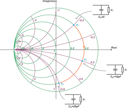
Figure 7. Example chart replacing the equivalent circuits of Figure 6.
As can be seen, by increasing the value of the parallel capacitor, the overall admittance moves along the constant-conductance circle in a clockwise direction.
Example 3: Adding a Parallel Inductor
The addition of a parallel inductor makes the susceptance component of the admittance more negative. For example, assume that the operating frequency is 222.82 MHz and Y0 = 20 mS. If we add a 71.42 nH parallel inductor to y1 = 0.2 - j0.5, the normalized susceptance component changes by -j0.5:
\[\begin{eqnarray}
jb &=& \frac{1}{ j2 \pi f LY_0} \\
&=& \frac{-j}{2 \pi \times 222.82 \times 10^6 \times 71.42 \times 10^{-9} \times 0.02}=-j0.5
\end{eqnarray}\]
This moves us to y2 = 0.2 - j, as shown in Figure 8.
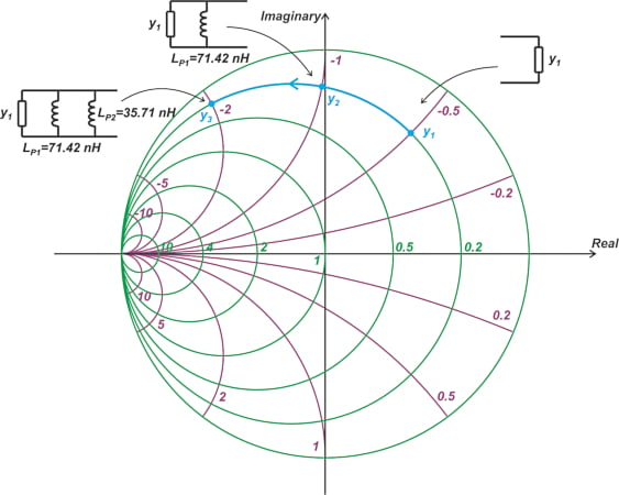
Figure 8. Smith chart showing the shift when adding a parallel inductor.
The figure also shows how adding another parallel inductor of Lp2 = 0.5 × 71.42 nH = 35.71 nH reduces the normalized susceptance by j1, producing an equivalent normalized admittance of 0.2 - j2. As can be seen, adding more and more series inductors moves us along a constant-conductance circle in a counterclockwise direction. If we replace the circuit schematics of Figure 8 with their equivalent circuits, we obtain the following equivalent diagram (Figure 9).
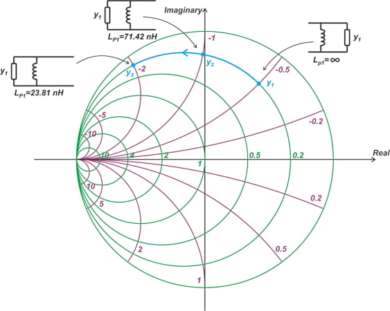
Figure 9. Example chart showing the addition of adding more inductors and replacing the circuit schematics of Figure 8 with their equivalent circuits.
The above diagram shows that if we reduce the value of a parallel inductor, the overall admittance moves along the corresponding constant-conductance circle in a counterclockwise direction.
Example 4: The Frequency Sweep of a Parallel RC Network
Next, let’s see how the admittance of a parallel RC circuit changes with frequency. Assume that R = 25 Ω, C = 10 pF, and Y0 = 20 mS. The normalized admittance of this parallel RC circuit is:
\[\begin{eqnarray}
y &=& \frac{1}{RY_0}+\frac{j \omega C}{Y_0} \\
&=& 2+j\frac{ \omega C}{Y_0}
\end{eqnarray}\]
The real part of the normalized admittance is g = 2. Therefore, the admittance of this circuit is on the constant-conductance circle of g = 2, and the susceptance is always positive. As the frequency is swept from DC to infinity, x changes from 0 to +∞. Thus, regardless of the value of the capacitor, the admittance locus includes the lower half of the g = 2 constant-conductance circle.
Note that since b changes from 0 to +∞ with frequency, we move clockwise along the circle as frequency increases. The cyan curve in Figure 10's curve shows the admittance locus on the Smith chart.
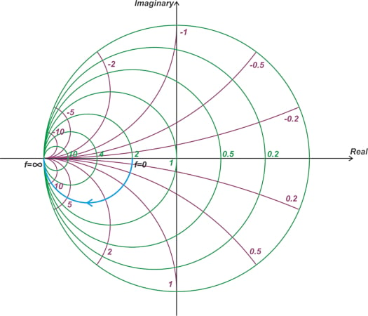
Figure 10. The admittance locus on the Smith chart.
Example 5: The Frequency Sweep of a Parallel RL Network
What would be the admittance contour of a parallel RL circuit with R = 25 Ω and L = 30 nH if we sweep the frequency from DC to infinity?
With Y0 = 20 mS, the admittance of this RL network is on the constant-conductance circle of g = 2. The susceptance component is \(b = - \frac{1}{L \omega Y_0}\), which is always negative. As the frequency is swept from DC to infinity, b changes from -∞ to 0. Therefore, regardless of the value of the inductor, the admittance locus includes the upper half of the g = 2 constant-conductance circle, as shown in Figure 11.
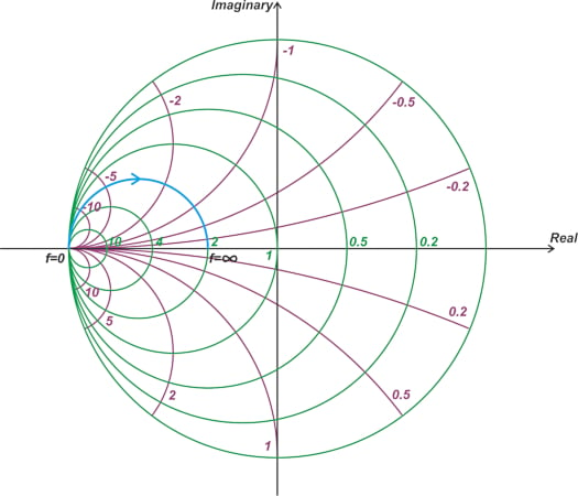
Figure 11. Smith chart showing the admittance locus, including the upper half of g = 2.
Note that since b changes from -∞ to 0 with frequency, we move clockwise along the circle as frequency increases.
Example 6: The Frequency Sweep of a Parallel RLC Network
As a final question, what would be the admittance contour of a parallel RLC circuit with R = 25 Ω and L = 20 nH, and C = 2 pF if we sweep the frequency from DC to infinity?
With Y0 = 20 mS, the admittance of this parallel RLC network is on the constant-conductance circle of g = 2. At the resonant frequency fr, the susceptance of the inductor cancels that of the capacitor, leaving us with a purely resistive admittance. Therefore, at fr, we are at the intersection of the g = 2 constant-conductance circle and the horizontal diagonal of the Smith chart (Figure 12).
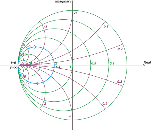
Figure 12. Smith chart showing fr at the intersection of g = 2 constant-conductance and the Smith chart's horizontal diagonal.
Below fr, the magnitude of the inductive susceptance is larger than the capacitive susceptance, and thus the circuit is inductive. This means that for 0 < f < fr, the circuit is capacitive, and we are at the lower half of the constant-conductance circle. On the other hand, for f > fr, the circuit is capacitive, and we are at the lower half of the constant-conductance circle. The above examples show that as frequency increases, the admittance contour always follows the constant-conductance circle in a clockwise direction.
Admittance Smith Chart Basics Summary
At a given frequency, a parallel RLC circuit can be represented by a single point on the admittance Smith chart. If the frequency is swept, the imaginary part of the admittance changes, and we obtain an admittance contour on the Smith chart that describes the circuit behavior. It is important to be familiar enough with the Smith chart to recognize what type of circuit configuration can produce a given admittance contour.
To see a complete list of my articles, please visit this page.