Facebook
 Google
 GitHub
 Linkedin
Transmission Line Theory: Observing the Reflection Coefficient and Standing Wave
Learn about radio frequency (RF) wave propagation and reflection via transmission lines, equations, and example waveforms.
Various types of waves in nature behave fundamentally alike. Like a voice that echoes off of a cliff, electrical waves reflect when they encounter a change in the impedance of the medium they are traveling in. Wave reflection can lead to an interesting phenomenon called the standing wave. Standing waves are essential to the way most musical instruments produce sound. For example, string instruments would not function without the predictability and amplification effects of the standing waves.
However, in RF design, standing waves are undesirable when we aim to transfer power from one block to the next one in the signal chain. In fact, standing waves can affect the performance of different RF and microwave systems, from anechoic chambers to everyday appliances such as microwave ovens.
While the concepts of wave propagation and reflection are not terribly complicated, they might be a little confusing at first. The best way to visualize how the waves propagate and reflect off of a discontinuity is to plot the wave equations for different configurations.
In this article, we’ll first derive the required equations and use them to explain the standing wave phenomenon through several example waveforms.
Transmission Line Voltage and Current Wave Equations
First, let’s derive our equations. I know it’s boring, but they really help us understand how waves propagate and interact with each other on a transmission line. In the previous article in this series, we examined the sinusoidal steady-state response of a transmission line and derived the voltage and current equations. Applying vs(t) = Vscos(ωt) to a line, the voltage and current waves are:
\[v(x,t)= A cos(\omega t-\beta x) + B cos(\omega t+\beta x)\]
\[i(x,t)=\frac{A}{Z_0} cos(\omega t-\beta x)- \frac{B}{Z_0} cos(\omega t+\beta x)\]
Where:
- A and B are constants that can be found from boundary conditions at the input and output ports of the line
- Z0 is the characteristic impedance
- β is the phase constant
These equations correspond to the configuration shown in Figure 1(a), where the positive x-axis direction is chosen to be from the source to the load. If we represent these waves with their phasors, the forward-traveling (or incident) wave and the backward-traveling (or reflected) voltage waves will be, respectively, Ae-jβx and Bejβx, as shown in Figure 1(a).
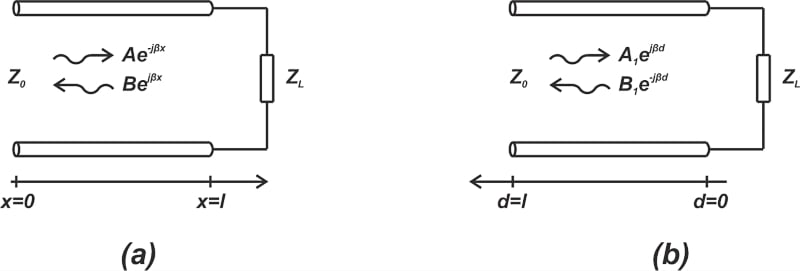
Figure 1. Diagrams showing the positive axis direction are from the source to the load (a) and then from the load to the source (b).
Regarding transmission line problems, it is usually more convenient to choose the positive axis direction from the load to the source, as shown in Figure 1(b). To find the new equations, we need to replace x in the original equations with l-d. As expressed in the new variable, d, the forward-traveling wave becomes:
\[Ae^{-j \beta x} = Ae^{-j \beta (l-d)}=Ae^{-j \beta l}e^{j \beta d} = A_1 e^{j \beta d}\]
Where A1 = Ae-jβl is a new constant. From here, you can verify that, in the new coordinate system, the reflected wave is B1e-jβd, where B1 = Bejβl. Therefore, the total voltage and current phasors are shown in Equations 1 and 2.
\[V(d)=A_1e^{j \beta d}+B_1e^{-j \beta d}\]
Equation 1.
\[I(d)=\frac{A_1}{Z_0}e^{j \beta d}-\frac{B_1}{Z_0}e^{-j \beta d}\]
Equation 2.
These equations make it easier to examine the load effect on the wave reflection because, in this case, the load is at d = 0, simplifying the equations. Letting d = 0, the following equations are obtained at the load end, as seen in Equations 3 and 4.
\[V(d=0)=A_1+B_1\]
Equation 3.
\[I(d=0)=\frac{A_1}{Z_0}-\frac{B_1}{Z_0}\]
Equation 4.
For example, let’s consider the case where the line is terminated in an open circuit. With the output open-circuited (ZL = ∞), the output current is obviously zero. From Equation 4, we have A1 = B1, and thus, the total voltage is V(d = 0) = 2A1.
Therefore, for an open circuit line, the reflected voltage is equal to the incident voltage at the output, and the total voltage at this point is double the incident voltage. Similarly, we can use Equations 3 and 4 to find the ratio of the reflected wave to the incident wave for an arbitrary load impedance ZL. This ratio is an important parameter known as the reflection coefficient, which we’ll get into shortly.
Input Impedance and Reflection Coefficient Formula
Using Equations 1 and 2, we can find the ratio of voltage to current (i.e., the input impedance of the transmission line) at different points along the line. This leads to Equation 5.
\[Z_{in}(d) = \frac{V(d)}{I(d)}=Z_0 \frac{A_1e^{j \beta d}+B_1e^{-j \beta d}}{A_1e^{j \beta d}-B_1 e^{-j \beta d}}\]
Equation 5.
Noting that the line impedance at the load end of the line (d = 0) is equal to the load impedance ZL, we obtain:
\[Z_L = Z_0 \frac{A_1+B_1}{A_1-B_1}\]
Using a little algebra, the above equation gives us the ratio of the reflected voltage wave to the incident voltage wave (B1/A1), which is defined as the reflection coefficient Γ in Equation 6.
\[\Gamma = \frac{Z_L - Z_0}{Z_L + Z_0}\]
Equation 6.
The above discussion shows that for a terminated line, there is a definite relationship between the incident and reflected waves. Note that, in general, a reflection coefficient is a complex number, and both magnitude and phase information of Γ are important. For power transfer, we attempt to have a matched load (ZL = Z0), leading to Γ = 0. Under this condition, a wave applied to the input is completely absorbed by the load, and no reflection occurs. It is instructive to consider two other special cases here: an open circuit line and a short circuit line that we’ll get into shortly.
While the concepts of wave propagation and reflection are not basically complicated, they might be confusing at first. The best way to visualize how the waves propagate and reflect off of a discontinuity is to plot the equations we have developed above. Also, it’s worth mentioning that there are many online simulators that might help you develop a better understanding of wave propagation concepts.
Short Circuit Lines
Next, let's go over short circuit lines. With a short circuit, the total output voltage should be zero at all times. Additionally, from Equation 6, we have Γ = -1. The incident voltage wave is given by:
\[v_i (d,t)=Real \text{ } Part \text{ }of \Big (A_1 e^{j \beta d} e^{j \omega t} \Big ) = A_1 cos(\omega t+\beta d)\]
The top curve in Figure 2 provides the plot of this equation at three different points in time t1, t2, and t3, where t1 < t2 < t3.
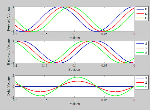
Figure 2. Example curves for the forward voltage (top), backward voltage (middle), and total voltage (bottom) of a short circuit.
The above curves breakdown where:
- The length of the transmission line is 0.2 meters
- The load is at d = 0
- β is 50 radian/meter
- The signal frequency is 2 GHz
Note how the incident wave gradually moves toward the load (at d = 0) as time passes. The middle curve in the above figure shows the reflected voltage that moves away from the load. The reflected voltage equation is:
\[v_r (d,t)=Real \text{ } Part \text{ }of \Big (\Gamma A_1 e^{-j \beta d} e^{j \omega t} \Big ) = A_1 cos(\omega t - \beta d)\]
Where Γ is set to -1 to take the short circuit into account. The total voltage is the sum of the incident and reflected voltages that are given in the lower curve. The forward voltage fluctuates between its minimum and maximum values at all points along the line, including the load end of the line. However, the reflected voltage takes the opposite value of the incident voltage so that the total voltage is always zero at the load end.
The total voltage wave has an interesting feature: it stands still, and unlike its constituent waves, the total voltage wave is not traveling in either direction. For example, the maximum and zero voltage points do not shift with respect to time. To better illustrate this, Figure 3 plots the total voltage for 36 different points in time.
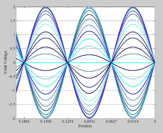
Figure 3. A plot showing the total voltage for 36 different points in time.
As can be seen, the zero-crossings (nodes) and the positions of maximum amplitude (antinodes) are some fixed positions along the line. Since the wave is not traveling in either direction, it is called a standing wave.
Open Transmission Circuit Line
For an open circuit line (ZL = ∞), Equation 6 yields Γ = 1. In this case, the magnitude and phase of the reflected voltage are equal to the incident voltage. The top and middle curves in Figure 4, respectively, show the incident and reflected voltage waves on an open circuit line at three different points in time.
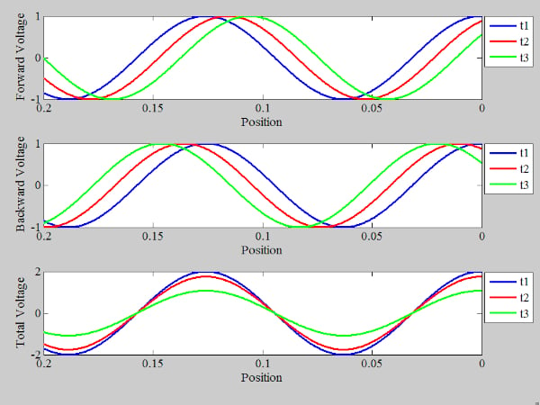
Figure 4. Example plots showing the forward voltage (top), backward voltage (middle), and total voltage (bottom) of an open circuit.
Note that both the incident and reflected waves have the same value at d = 0. Therefore, the total voltage (the bottom curve) is double the incident voltage at the load end. Since Γ = 1, the reflected current Ir also has the same magnitude and phase as the incident current Ii. However, the total current is Ii - Ir = 0 at the load end, which is no big surprise as the load is an open circuit.
Furthermore, we can again observe that the total voltage is a standing wave. This is best illustrated in Figure 5, which plots the total voltage wave for 36 different points in time.
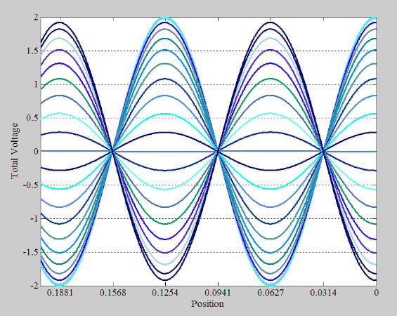
Figure 5. Example plot showing the total voltage wave for 36 different points in time for an open circuit.
Calculating an Arbitrary Load of a Terminated Line
Next, let’s use our equations to examine a terminated line with Γ = 0.5. The incident and reflected voltage waves at an arbitrary time are plotted in Figure 6.
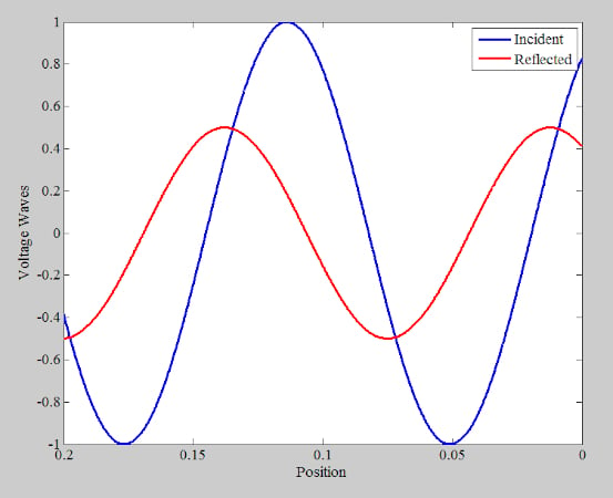
Figure 6. Plot showing the incident and reflected voltage waves.
These two waves are traveling in opposite directions. You should be able to imagine that at a certain point in time and at some specific position along the line, the peaks of the two waves will coincide, producing the maximum value of the total voltage wave. This is illustrated in Figure 7.
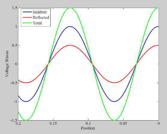
Figure 7. Example plot showing the maximum value of the total voltage wave when the peaks of the incident and reflected waves coincide.
Also, at some other point in time, a particular position along the line will “see” the peak of the larger wave and the minimum of the smaller one, as shown in Figure 8.
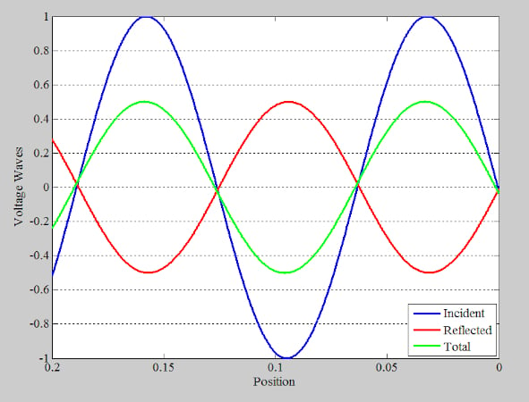
Figure 8. Example plot showing the total voltage wave where the incident and reflected waves have opposing peaks and valleys.
At these points, the amplitude of the total voltage wave is at its minimum. In our example, the forward and reflected waves respectively have an amplitude of 1 and 0.5. Therefore, the total voltage wave has a minimum amplitude of 1 - 0.5 = 0.5. To better observe the voltage amplitude at different points along the line, Figure 9 plots the total voltage wave at 36 different instances.
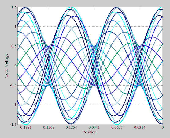
Figure 9. Example plot showing the total voltage wave at 36 different instances.
This figure gives you an idea of the fluctuation amplitude at different points on the line. Note that while points such as d = 0.1881 m fluctuate between ±1.5 V, there are other points. For example, d = 0.1568 m, which has a much smaller amplitude and fluctuates between ±0.5 V.
One question you might ask is, is the total wave traveling or standing still? Figure 10 shows a smaller number of the total voltage plots at some consecutive points in time (t1 < t2 < ...< t6) to answer this question.
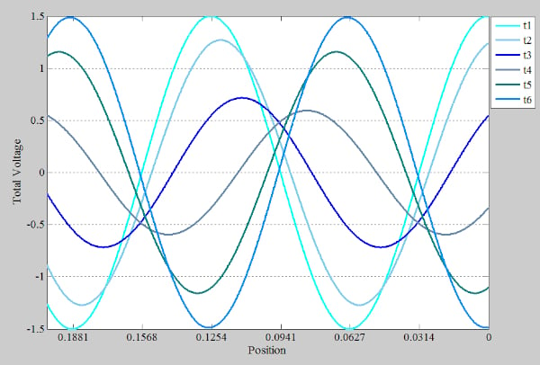
Figure 10. Example showing fewer total voltage plots at consecutive points in time.
The figure shows that, as time passes, the wave travels toward the load. Note that while the amplitude of the incident and reflected waves are constant, the amplitude of the combined voltage rises and falls over time.
Incident, Reflection, and Standing Waves Summary
Let’s summarize our observations:
- With a matched load, the incident wave travels toward the load, and there is no reflection. In this case, the wave has constant amplitude along the line.
- With short circuit and open circuit lines, the incident wave is totally reflected (Γ = -1 or 1). In this case, the combined voltage is not traveling in either direction and is called a standing wave.
- With standing waves, we have nodes and antinodes at fixed positions along the line. Nodes don’t fluctuate at all, whereas antinodes fluctuate at the maximum amplitude.
- With loads other than the above three cases, we have a traveling wave that rises and falls over time (although it is actually a traveling wave, we might still glibly occasionally refer to this wave as a standing wave). In this case, we don’t have any nodes, but some points have a smaller amplitude than others. This situation is between the ideal case of no reflection (Γ = 0) and the worst case of total reflection (Γ = ±1).
Therefore, with all that in mind, it is important for us to know at which point across this spectrum our transmission line is operating. The parameter VSWR (voltage standing wave ratio), which is defined as the ratio of the wave's maximum amplitude to its minimum amplitude, allows us to characterize how close we are to having a standing wave. When there’s total reflection, VSWR is infinite; for a matched load, VSWR is 1.
As for other cases, VSWR is somewhere between these two extreme values. The VSWR provides us with an alternative way of characterizing the amount of reflection. This will be discussed in greater detail in the next article.
To see a complete list of my articles, please visit this page.
Related Content