Understanding Matching Networks

Learn about why matching networks are used and how they are designed.

Back in Chapter 3, we discussed characteristic impedance, transmission lines, and impedance matching. We know that transmission lines have a characteristic impedance and we know that this impedance is an important factor in RF circuitry, because impedances must be matched to prevent standing waves and to ensure efficient transfer of power from source to load. And even if we don’t need to treat a particular conductor as a transmission line, we still have source and load impedances that need to be matched.

Also in Chapter 3, we saw that impedance matching is greatly simplified by the use of standardized impedance values (the most common being 50 Ω). Manufacturers design their components or interconnects for 50 Ω input and output, and in many cases an engineer does not have to take any specific action to achieve matched impedances.

However, there are situations in which impedance matching requires additional circuitry. For example, consider an RF transmitter composed of a power amplifier (PA) and an antenna. The manufacturer can design the PA for 50 Ω output impedance, but the impedance of an antenna will vary according to its physical characteristics as well as the characteristics of the surrounding materials.

Also, the antenna’s impedance is not constant relative to signal frequency. Thus, a manufacturer could design an antenna that has 50 Ω impedance at one specific frequency, but you might have a nontrivial mismatch if you use the antenna at a different frequency. The following plot is taken from the datasheet for a ceramic surface-mount antenna intended for 2.4–2.5 GHz systems. The curve corresponds to the ratio of reflected power to incident power. You can see that the quality of the impedance match deteriorates rapidly as the signal frequency moves away from 2.45 GHz.

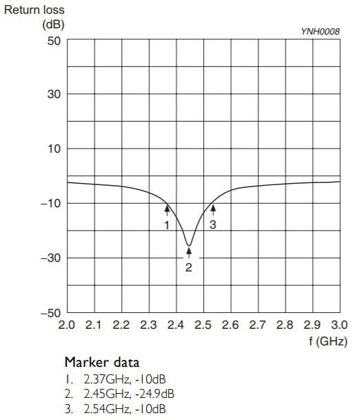
Plot taken from this datasheet.

The Matching Network

If your RF circuit contains components that do not have matched impedances, you have two options: modify one of the components, or add circuitry that corrects the mismatch. Nowadays the first option is generally not practical; it would be difficult indeed to adjust impedance by physically modifying an integrated circuit or a manufactured coaxial cable. Fortunately, though, the second option is perfectly adequate. The additional circuit is called a matching network or an impedance transformer. Both names are helpful in understanding the fundamental concept: a matching network enables proper impedance matching by transforming the impedance relationship between source and load.

The design of matching networks is not particularly simple, and it’s not something that we will discuss thoroughly in a textbook such as this one. Nonetheless, we can consider some of the basic principles, and we’ll also take a look at a fairly straightforward example. Here are some salient points to keep in mind:

• A matching network is connected between a source and a load, and its circuitry is usually designed such that it transfers almost all power to the load while presenting an input impedance that is equal to the complex conjugate of the source’s output impedance. Alternatively, you can think of a matching network as transforming the output impedance of the source such that it is equal to the complex conjugate of the load impedance.
  • (In real-life circuits the source impedance often has no imaginary part, and thus we don’t need to always refer to the complex conjugate. We can simply say that the load impedance must equal the source impedance, because the complex conjugate isn’t relevant when the impedance is purely real.)
• Typical matching networks (referred to as “lossless” networks) use only reactive components, i.e., components that store energy rather than dissipate energy. This characteristic follows naturally from the purpose of a matching network, namely, to enable maximum power transfer from source to load. If the matching network contained components that dissipate energy, it would consume some of the power that we are trying to deliver to the load. Thus, matching networks use capacitors and inductors, and not resistors.
• It is difficult to design a wideband matching network. This is not surprising when we remember that the matching network is composed of reactive components: the impedance of inductors and capacitors is dependent on frequency; thus, changing the frequency of the signals passing through the matching network can cause it to be less effective.

The L Network

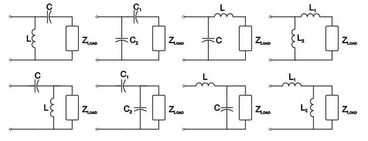
The most straightforward matching-network topology is called the L network. This refers to eight different L-shaped circuits composed of two capacitors, two inductors, or one capacitor and one inductor. The following diagram shows the eight L-network configurations:

The L network is simple and effective, but it is not suitable for wideband applications. We also have to keep in mind that inductors and capacitors exhibit seriously nonideal behavior at high frequencies (as discussed in Page 4 of Chapter 1), and thus the behavior of the L network will be less predictable as frequencies climb into the gigahertz range.

It is certainly valuable to understand the concepts involved in manually calculating matching-network values based on the source and load impedances, though this is more of an academic or intellectual exercise in an age when calculator tools can readily accomplish this task. We won’t go through a calculation example here, but we will use a simulation to explore the effects of a matching network.

An Example

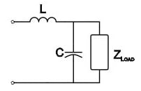
Let’s say that we have a source impedance of 50 Ω and an antenna impedance of 200 Ω, and we are operating at 100 MHz. We’ll use an L network consisting of an inductor followed by a capacitor:

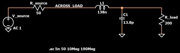
AAC’s L-network design tool gives the following values for the inductor and capacitor: 138 nH and 13.8 pF. This means that our impedance-matched circuit looks like this:

To evaluate the efficacy of the matching network, we can run a simulation and then plot the voltage across the load divided by the current flowing into the load, which is equal to the input impedance. (In this case the current flowing into the load is the current through inductor L1.) An AC analysis is particularly helpful because we can see how the effect of the matching network changes with frequency. The following plot is for a simulation with a frequency range of 10 MHz to 190 MHz (i.e., 90 MHz above and below the frequency for which the matching network was designed). Here are the results:

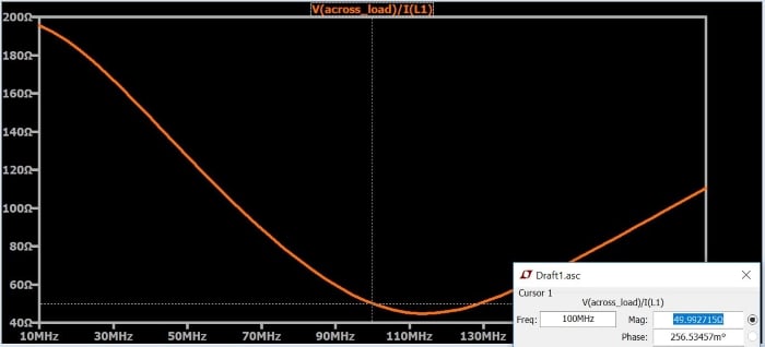
As you can see, at 100 MHz the load is very closely matched to the 50 Ω source impedance, despite the fact that the original load has an impedance of 200 Ω. However, we said above that the L network is not a wideband topology, and the simulation certainly confirms this: the input impedance changes rapidly as the signal frequency moves away from 100 MHz.

Summary

• A matching network, also called an impedance transformer, is used to create matched impedance between a source and a load (for example, between a power amplifier and an antenna).
• Lossless matching networks consist of reactive components only; resistive components are avoided because they would dissipate power, whereas the matching network is intended to facilitate the transfer of power from source to load.
• A straightforward, narrowband matching-network topology is the L network. It consists of two reactive components.
• Calculator tools can be used to quickly design a matching network based on the source impedance, load impedance, and signal frequency.