Use the Xilinx CORDIC Core to Easily Generate Sine and Cosine Functions

This article will review integrating a Xilinx IP core into an FPGA design.

We’ll add the CORDIC core to generate sine and cosine of a given angle. The process of using the Xilinx Core Generator tool will be discussed. The article will also review some basic properties of the Xilinx CORDIC core.

Use Code Segments developed by Sophisticated Engineers

In a previous article, we saw that VHDL components allow us to have a neat hierarchical design and reuse a previously developed code segment several times. We can also use this capability of hardware description languages to add optimized code segments which are developed by experienced engineers to our design. Such a ready-made component is called a core.

You can find cores for a wide variety of functions, such as multipliers, digital filters, DSP-related transforms, memories and more. Since cores are generally optimized and verified, you don’t have to worry about their performance. As a result, you can concentrate on the rest of your design and finish your project much faster.

There are two types of cores that can be used with Xilinx products: LogiCORE and AllianceCORE solutions. LogiCORE solutions are developed by the experts working for Xilinx; however, the experts that develop AllianceCOREs are not employed by Xilinx. Many of the LogiCORE components are provided for free with the Xilinx software packages. In this article, we’ll add the Xilinx LogiCORE IP CORDIC v4.0 to an ISE design and use it to calculate the sine and cosine of a given angle.

Choose a Core

To add a core to your ISE project, click on “New Source” under the “Project” tab and choose “IP (CORE Generator & Architecture Wizard)” as shown in Figure 1.

 

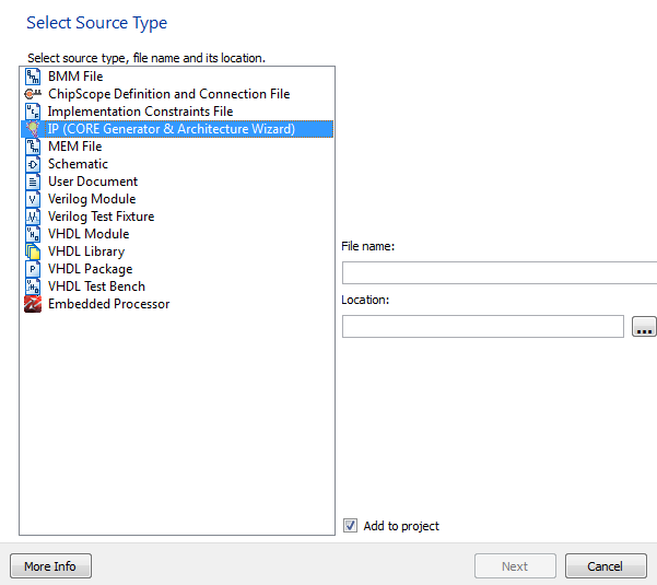
Figure 1

 

Give your file a name and location and click on “Next”. Then, you’ll see a list of the available cores. We’ll choose “CORDIC 4.0” as shown in Figure 2.

 

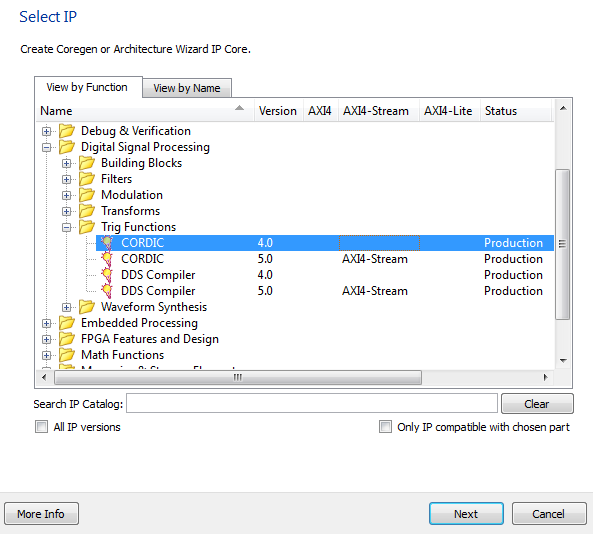
Figure 2

 

Then, a GUI will open which allows you to customize the core according to your needs.

Set the Parameters of the Core

For the CORDIC core, there are three pages of settings. The first page is shown below:

 

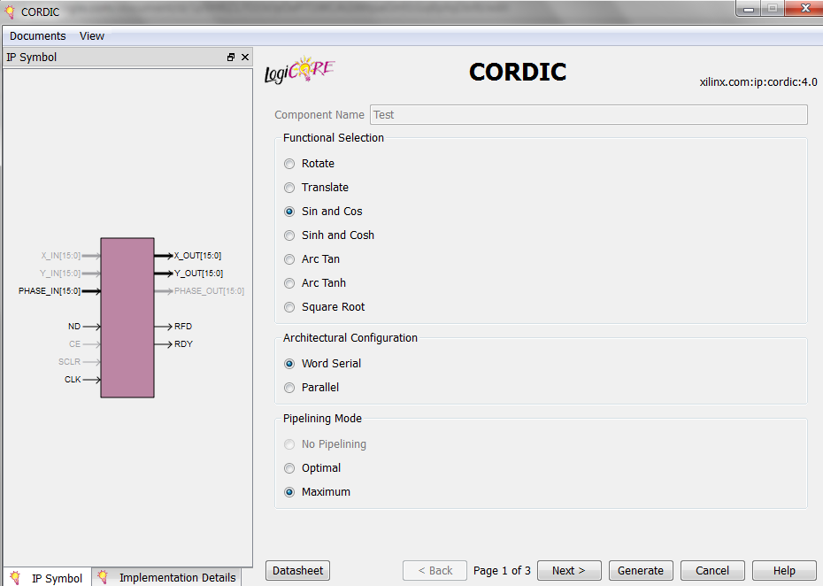
Figure 3

 

The GUI shows a symbol for the core where you can see the active inputs and outputs of the core. Note that, based on the chosen features of the core, a terminal may or may not be active.

By clicking on the “Datasheet” button, you can access a document that covers different options of the core in detail. It also has a brief review of the CORDIC theory. In this article, we’ll explain different features of the core as much as needed. For more details, please read the datasheet.

The “Functional Selection” allows us to choose the function that we want to implement. As discussed in a previous article introducing the CORDIC algorithm, there are several functions that can be implemented using the CORDIC algorithm. In this article, we want to realize the sine and cosine functions, so we choose “Sin and Cos”.

The “Architectural Configuration” specifies the structure used to implement the CORDIC algorithm. The “Word Serial” architecture sequentially uses a single shift-add/subtract stage to perform the iterations of the algorithm. That’s why it is area efficient. However, after applying the inputs, we’ll have to wait several clock cycles before the core generates a new output.

On the contrary, the “Parallel” architecture uses an array of shift-add/subtract stages and offers a much higher speed at the cost of increased hardware. For this example, we’ll use a “Word Serial” architecture.

The “Pipelining Mode” allows us to use a pipelined implementation. Some options of the “Pipelining Mode” may become inactive because of the function and architecture that we choose. For example, in Figure 3, the “No Pipelining” option is inactive. We’ll keep the default option for the “Pipelining Mode” which is “Maximum”.

By clicking on the “Next” button, the second page of settings will appear as shown in Figure 4.

 

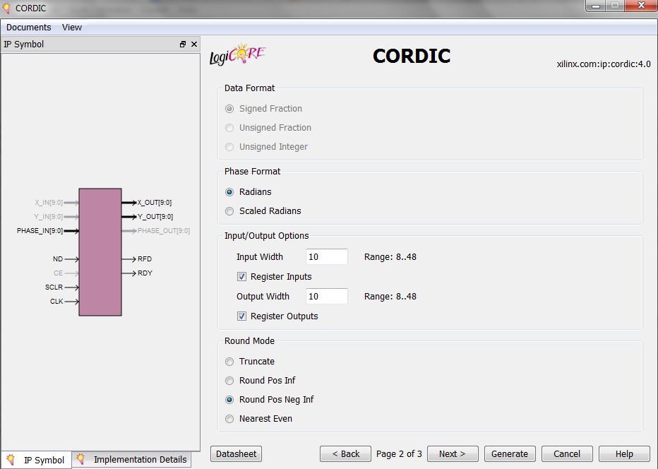
Figure 4

When using the CORDIC algorithm to implement sine and cosine functions, we have a phase input, PHASE_IN which is an angle, and two outputs, X_OUT and Y_OUT, which give the cosine and sine of PHASE_IN, respectively. These input/outputs are shown in the core symbol above. For more details about using the CORDIC algorithm to calculate the sine and cosine functions read my previously mentioned article on the CORDIC algorithm.

The second page of the core settings includes some options to specify how the inputs/outputs will represent the data. The first part of page 2, “Data Format”, determines the way X and Y inputs/outputs are expressed. In our case, the “Data Format” will specify the format of X_OUT and Y_OUT.

As you can see from Figure 4, with the settings that we’ve chosen so far, the “Data Format” will be the default which is “Signed Fraction”. Referring to the datasheet, we see that X_OUT and Y_OUT will be expressed as fixed-point 2’s complement numbers with an integer width of two bits. Note that the integer width is 2 bits but the overall width of the outputs can be specified by the “Output Width” in Figure 4. In our example, the “Output Width” is chosen to be 10 bits. Hence, if the output data is 0010110101, we know that the binary point is between the eighth and ninth bits and we have $$00.10110101_2 = 0.70703125_{10}$$. Since the numbers are signed, the leftmost bit is the sign bit.

The next part of the page specifies the format for the phase input/output. For the “Sin and Cos” mode, we have the phase input PHASE_IN. Choosing the “Radians” option, the PHASE_IN will be considered as a fixed-point 2’s complement number with an integer width of three bits. Note that the overall width of the input will be determined by the “Input Width” in Figure 4. Hence, if PHASE_IN is “0000101011”, the input angle will be $$000.0101011_2 = 0.3359375_{10}$$ radians. As shown in Figure 4, we’ll use the core with registered inputs and outputs.

For the rounding mode, we’ll choose “Round Pos Neg Infinity” which is equivalent to the MATLAB function round(x). You can find examples of the different rounding modes in the core datasheet. The third page of the settings is shown in Figure 5.

 

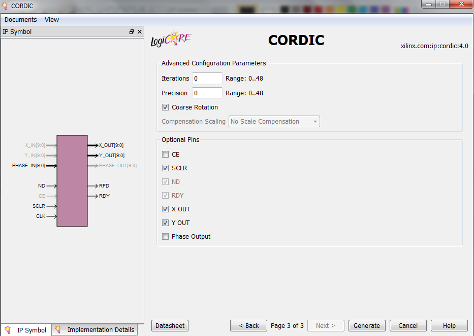
Figure 5

On this page, we can choose the number of iterations for the CORDIC algorithm and the internal precision for the add/subtract operations. According to the datasheet, setting the value of these two options to zero will force the software to automatically figure out these two parameters based on the accuracy of the outputs and other parameters. We’ll keep these parameters as they are by default.

 The last part specifies the optional pins of the core. We’ll add the “SCLR” input which stands for synchronous clear. When “SCLR” is asserted all the core flip-flops are synchronously initialized.

Pushing the “Generate” button will produce an .xco file and add the core to the design. By clicking on this file and then choosing “View HDL Instantiation Template” in the ISE software, you can find the template to declare the component of the core. Now, you can use this component just as you use a normal VHDL component.

ISE Simulation

To use the core, you’ll need to study the “Control Signals and Timing” section of the datasheet. Figure 6 shows how the control signals of the CORDIC core must be used when a “Word Serial” structure is chosen for the core.

 

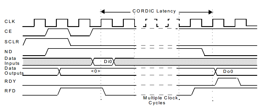
Figure 6

 

The “SCLR” input is asserted to initialize all the core flip-flops. Now, we can apply the input data and set the “New Data” input, i.e. “ND”, to logic high so that the core is allowed to sample the input data on the next rising clock edge.

When the calculations are done, the core will set the “RDY” output to logic high to indicate that valid outputs are generated. The core will also set the “Ready For Data” output, i.e. “RFD”, to logic high to indicate that the module is ready to sample new input data.

Figure 7 shows an ISE simulation of our CORDIC core. This simulation uses a set of waveforms similar to that of Figure 6.

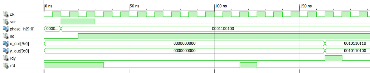
Figure 7

 

As you can see, the input, PHASE_IN, is $$0001100100_2 = 000.1100100_2 = 0.78125_{10}$$ radians. Hence, we expect X_out=cos(0.78125)=0.70915311 and Y_out=sin(0.78125)=0.70416751. The simulation gives X_out=$$00.10110110_2 = 0.7109375_{10}$$ and Y_out=$$00.10110100_2 = 0.70312500_{10}$$. Increasing the “Output Width” will lead to a better accuracy.

Conclusion

You can find optimized and verified cores for a wide variety of functions, such as multipliers, digital filters, DSP-related transforms, memories and more. These ready-made cores allow you to approach a large design much more easily and finish your project much faster. The article showed that we can use the Xilinx CORDIC core easily and add sine and cosine functions into our FPGA design.

 

To see a complete list of my articles, please visit this page.