 Facebook
 Google
 GitHub
 Linkedin
How to Use Your Computer to Generate Complex Analog Waveforms
This article presents Scilab code that allows you to generate I/Q, noise, and chirp signals from your PC’s headphone jack.
This article presents Scilab code that allows you to generate I/Q, noise, and chirp signals from your PC’s headphone jack.
In my previous article, we discussed how to use your computer as an arbitrary wave generator via a technique whereby numerical signals are created in a computational program such as Scilab or MATLAB and then converted into analog signals via the computer’s audio hardware. This is a convenient and simple way to generate analog signals that have easily adjustable frequency and amplitude.
However, audio hardware is (quite reasonably) designed for audio frequencies, so we have to accept the limited bandwidth. We certainly won’t be generating RF signals directly from the headphone jack.
The previous article provided Scilab code for generating a basic sinusoid and a triangle wave. In this article, I want to further explore this topic using some signals that are a bit more interesting than what we’ve covered so far.
Before moving on, consider catching up with some of our related resources below:
Related Information
- How to Build Your Own Function Generator Using Analog Devices’ AD9833
- How to Generate a High-Precision Waveform Using a DAC and a Custom PCB
Previous Articles on Scilab-Based Digital Signal Processing
- Introduction to Sinusoidal Signal Processing with Scilab
- How to Perform Frequency-Domain Analysis with Scilab
- How to Use Scilab to Analyze Amplitude-Modulated RF Signals
- How to Use Scilab to Analyze Frequency-Modulated RF Signals
- How to Perform Frequency Modulation with a Digitized Audio Signal
- Digital Signal Processing in Scilab: How to Remove Noise in Recordings with Audio Processing Filters
- Audio Processing in Scilab: How to Implement Spectrum Subtraction
- Digital Signal Processing in Scilab: How to Decode an FSK Signal
- Digital Signal Processing in Scilab: Understanding Phase Misalignment in FSK Decoding
- How to Use I/Q Signals to Design a Robust FSK Decoder
- How to Process I/Q Signals in a Software-Defined RF Receiver
- How to Use Your Computer as an Arbitrary Waveform Generator
Generating I/Q Signals
I’ve written quite a bit about the use of I/Q signals. Two of the articles in the Scilab DSP series provide detailed information on the benefits and implementation details of I/Q signals in the context of a specific application, and this page in AAC’s RF textbook explains how phase modulation can be achieved by varying the amplitudes of I/Q signals and then adding them together. The bottom line is that I/Q techniques are fundamental aspects of signal processing and can greatly improve the performance of communication systems.
That being said, I’m really glad that at some point people insisted upon having two separate channels—i.e., Left and Right—in audio systems. Not because of the improved listening experience (I much prefer music that comes “straight from the instrument,” so to speak), but because the Left and Right channels provide such a convenient way to implement I/Q signal generation.
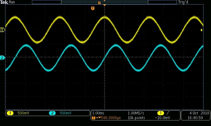
Thus far the input argument to the sound() function has been an array (or to use Scilab’s terminology, a vector). This array contains one series of values that corresponds to one signal, and this one signal will be sent to both audio channels. However, the input argument can also be a matrix consisting of two arrays, and in this case the signal corresponding to the first array becomes the Left audio and the signal corresponding to the second array becomes the Right audio. The following Scilab commands give you an example of I/Q signal generation using the sound() function.
SignalFrequency = 441;
SamplingFrequency = 22.05e3;
Samples_per_Cycle = SamplingFrequency/SignalFrequency;
n = 0:(Samples_per_Cycle-1);
Signal_OneCycle_I = cos(2*%pi*n / (SamplingFrequency/SignalFrequency));
Signal_OneCycle_Q = sin(2*%pi*n / (SamplingFrequency/SignalFrequency));
CycleDuration = (1/SamplingFrequency) * length(n);

FullSignal_I = 0;
FullSignal_Q = 0;
for k=1:(10/CycleDuration)
  > FullSignal_I = [FullSignal_I Signal_OneCycle_I];
  > FullSignal_Q = [FullSignal_Q Signal_OneCycle_Q];
  > end


FullSignal_IQ = [FullSignal_I; FullSignal_Q];
sound(FullSignal_IQ)
Making Noise
Many electrical engineers devote a significant portion of their life to suppressing noise. Consequently, there’s something strange—cathartic, even—about intentionally creating noise. Catharsis is not the only reason for generating a noisy signal, though. It also helps you to determine how a circuit will respond to a specific type of noise.
Let’s say you have a sensor circuit that will occasionally be subjected to high-frequency interference from a nearby device. To determine how this noise will affect the output of the sensor’s amplifier, you could model the noise in Scilab and superimpose it on a waveform that resembles the amplifier’s input signal. This numerical version of the noisy input signal can then be converted into an analog waveform and delivered to the actual amplifier circuit.
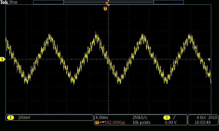
The following Scilab commands provide an example of noisy-signal generation. The input signal is a 110.25 Hz triangle wave, and the noise is composed of two smaller-amplitude sinusoids at 2 kHz and 3.5 kHz.
SignalFrequency = 110.25;
SamplingFrequency = 22.05e3;
Samples_per_Cycle = SamplingFrequency/SignalFrequency;
n = 0:(Samples_per_Cycle-1);
CycleDuration = (1/SamplingFrequency) * length(n);
LowerLimit = -1;
UpperLimit = 1;
StepSize = (UpperLimit - LowerLimit)/(length(n)/2);
UpwardRamp = LowerLimit:StepSize:(UpperLimit - StepSize);
DownwardRamp = UpperLimit:-StepSize:(LowerLimit + StepSize);
TriangleWave_OneCycle = [UpwardRamp DownwardRamp];
TriangleWave_Full = 0;


NoiseFrequency1 = 2e3;
NoiseFrequency2 = 3.5e3;
NoiseComponent1 = 0.1*sin(2*%pi*n / (SamplingFrequency/ NoiseFrequency1));
NoiseComponent2 = 0.1*sin(2*%pi*n / (SamplingFrequency/ NoiseFrequency2));
NoisySignal_OneCycle = TriangleWave_OneCycle + NoiseComponent1 + NoiseComponent2;

NoisySignal_Full = 0;
for k=1:(10/CycleDuration)
  > NoisySignal_Full = [NoisySignal_Full NoisySignal_OneCycle];
  > end
sound(NoisySignal_Full)
The Chirp Signal
A handy way to determine the frequency response of a physical circuit is to provide an input signal that rapidly increases (or decreases) in frequency. You can then look at the output waveform on an oscilloscope and observe the relationship between frequency and amplitude, and you could even create a Bode plot by measuring the amplitude at various frequencies and plotting the results.
A waveform that exhibits this sort of intentional, steady increase or decrease in frequency is called a chirp signal (other options are “sweep signal” and “frequency-sweep signal”). Creating easily adjustable chirp signals using analog circuitry is not what I would describe as a straightforward task, but our Scilab/MATLAB-to-analog system makes the design process fast and relatively simple.
The Scilab commands given below will generate a chirp signal that starts at 10 Hz and ends at approximately 10 kHz. The method of increasing the frequency is as follows:
- The initial period is 1/(10 Hz) = 0.1 ms. The changes in frequency occur relative to this initial period.
- I want each frequency to complete an integer number of sine-wave cycles, i.e., the sine waveform for each frequency must begin at zero and end at zero. This ensures that the chirp signal doesn’t have discontinuities, which create spurious high-frequency content.
- After each length of time corresponding to the initial period, the frequency is increased by a factor of two. This allows us to cover the frequency range quickly and avoids discontinuities by causing every frequency to be an integer multiple of the minimum frequency.
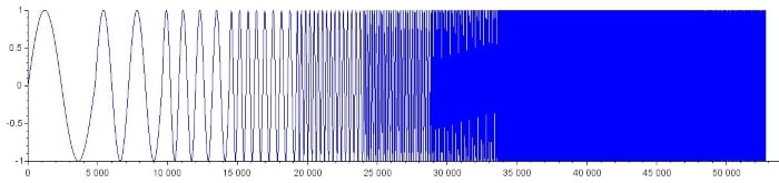
MinimumFrequency = 10;
MaximumFrequency = 10e3;
SamplingFrequency = 48e3;
Samples_per_Cycle = SamplingFrequency/MinimumFrequency;
n = 0:(Samples_per_Cycle-1);
Chirp = 0;
InstantaneousFrequency = MinimumFrequency;
Chirp = sin(2*%pi*n / (SamplingFrequency/InstantaneousFrequency));
while (InstantaneousFrequency < MaximumFrequency)
  > InstantaneousFrequency = InstantaneousFrequency * 2;
  > Waveform_at_NextFrequency = sin(2*%pi*n / (SamplingFrequency/InstantaneousFrequency));
  > Chirp = [Chirp Waveform_at_NextFrequency];
  > end
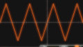
This is what the chirp signal looks like in Scilab:
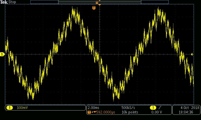
And here are two scope captures:
sound(Chirp, 48e3)

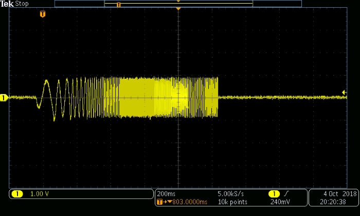
(It appears that the audio hardware has an inverting amplifier on the output of the DAC—note how the Scilab chirp starts with a positive slope, as we would expect with a normal sine wave, but the analog chirp starts with a negative slope.)
Other Signals You'd Like to See?
Now we've generated some interesting analog waveforms using Scilab and a typical PC headphone jack. If you have any ideas for other useful signals that could be generated using this method, let us know in the comments section below.
Related Content


I’ve learned a lot of new things here. Enjoyed reading this.
Thanks so much for this easy and simple explanation of all the essential suggestions for writing an article .
http://smtinsight.com
I’ve learned a lot of new things here. Enjoyed reading this.
Thanks so much for this easy and simple explanation of all the essential suggestions for writing an article .
http://smtinsight.com
I’d like to see how to make “square” waves in the 40 to 200 Hz range along with programmed variable amplitude.