How to Use Your Computer as an Arbitrary Waveform Generator

Learn how your computer can function as an arbitrary waveform generator. In this article, we’ll use Scilab to generate numerical signals that can be converted into analog waveforms by a computer’s audio hardware.

Lately I have been writing articles that demonstrate the use of Scilab for various signal-processing tasks. DSP experimentation in this sort of computational environment is extremely convenient; algorithms involved in communication, sensor, and audio systems can be quickly developed and refined, and signals can be carefully analyzed in the time domain and the frequency domain.

The next step is to extend all of this signal-processing activity into the realm of real voltage signals, and Scilab makes it very easy to accomplish this (I’m assuming here that your computer can play sound). I don’t currently have access to MATLAB, but I assume that it provides equivalent functionality, so I’m hoping that almost everything in this article will be relevant for MATLAB users as well. There is another free MATLAB alternative called GNU Octave. I have never used it, so I would appreciate any input from Octave users regarding how to implement the digital-to-analog operations discussed in this article and the following article.

There are probably quite a few ways to make use of this Scilab-to-analog (or MATLAB-to-analog) functionality. One possibility that comes to mind is testing the high-frequency portion of a wireless transmitter by generating baseband signals in Scilab and converting them to analog signals that are connected to the RF circuitry. In this article, though, we will focus on a more generic application: using a typical computer as an arbitrary waveform generator.

Before moving on in this article, consider checking out resources and previous articles related to this topic:

Related Information

• How to Build Your Own Function Generator Using Analog Devices’ AD9833
• How to Generate a High-Precision Waveform Using a DAC and a Custom PCB

Previous Articles on Scilab-Based Digital Signal Processing

• Introduction to Sinusoidal Signal Processing with Scilab
• How to Perform Frequency-Domain Analysis with Scilab
• How to Use Scilab to Analyze Amplitude-Modulated RF Signals
• How to Use Scilab to Analyze Frequency-Modulated RF Signals
• How to Perform Frequency Modulation with a Digitized Audio Signal
• Digital Signal Processing in Scilab: How to Remove Noise in Recordings with Audio Processing Filters
• Audio Processing in Scilab: How to Implement Spectrum Subtraction
• Digital Signal Processing in Scilab: How to Decode an FSK Signal
• Digital Signal Processing in Scilab: Understanding Phase Misalignment in FSK Decoding
• How to Use I/Q Signals to Design a Robust FSK Decoder
• How to Process I/Q Signals in a Software-Defined RF Receiver

The Basic Setup

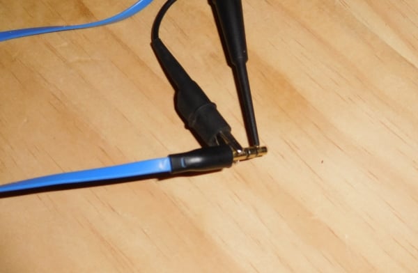
The only hardware you need is an audio cable with male connectors on both ends. One side plugs into the computer’s headphone port, and the other side delivers the signal to the relevant circuitry (or to an oscilloscope). The following photo shows how I clipped my Tektronix scope probe to the audio connector.

 

 

The command that we’ll be using to generate analog waveforms is called sound(). The only required input argument is the array of numbers that you want to send to the computer’s audio DAC. The values in this array must be greater than or equal to –1 and less than or equal to +1. This is convenient if you’re working with sinusoidal signals, because the sin() and cos() functions generate signals in this range. In general, though, you need to be aware of your signal amplitudes and scale as necessary into the range [–1, 1].

The sound() function also accepts an argument for the desired sample rate. If you don’t specify a sample rate, it uses the default value, which is 22.05 kHz.

While we’re on the subject of sample rate, I should mention the serious limitation that affects any attempt to use a computer’s audio hardware as a waveform generator. This hardware is intended for audio signals, and consequently its maximum sample rate has been chosen according to the audio quality that the hardware is intended to achieve. My impression is that nowadays many computers will support sampling frequencies up to 192 kHz, but it’s difficult to find clear information on the subject.

Generating a Sinusoid

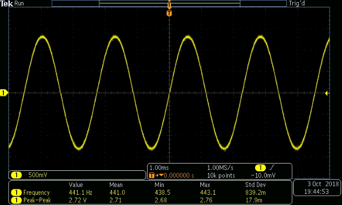
Let’s start with a simple example. We’ll generate a 441 Hz sinusoid and look at some scope captures.

 

SignalFrequency = 441;
SamplingFrequency = 22.05e3;
Samples_per_Cycle = SamplingFrequency/SignalFrequency;
n = 0:(Samples_per_Cycle-1);
Signal_OneCycle = sin(2*%pi*n / (SamplingFrequency/SignalFrequency));

 

The array n, and consequently also the Signal_OneCycle array, has a length of 50. The sampling period is 1/22050 ≈ 45 µs. Thus, one cycle lasts for approximately 50 × 45 µs = 2.25 ms. I like to have a duration of about ten seconds, so that I have plenty of time to look at the signal on the scope. The following for loop is used to extend the Signal_OneCycle array into an array with a length that corresponds to the desired signal duration.

 

CycleDuration = (1/SamplingFrequency) * length(n);
FullSignal = 0;
for k=1:(10/CycleDuration)
  > FullSignal = [FullSignal Signal_OneCycle];
  > end

 

Now we’re ready to generate the signal. We don’t have to specify the sample rate because the sampling frequency that I used (22.05 kHz) is the same as the default.

 

sound(FullSignal)

 

The following scope capture shows the generated waveform. At the bottom, you can see measurements for the peak-to-peak amplitude and the frequency. The amplitude direct from the headphone jack would probably be adequate for many applications; if you need higher voltages, a simple op-amp circuit would suffice.

 

 

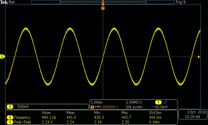
One particularly handy aspect of generating analog signals in this way is that the computer’s volume-adjustment functionality gives you excellent control over the amplitude of the signal. The following scope captures give you an idea of the relationship between amplitude and my computer’s audio volume.

 

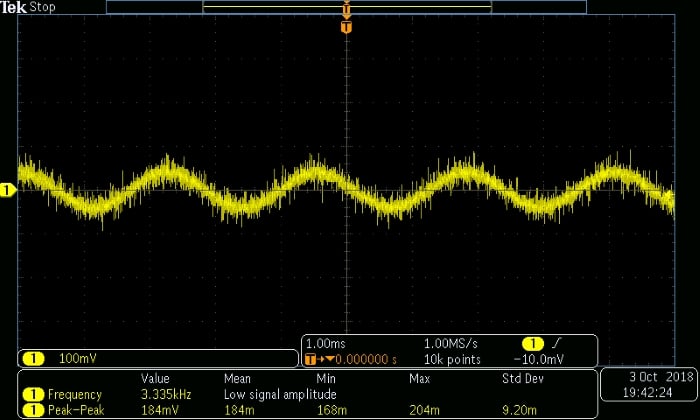
Volume setting: 10%

 

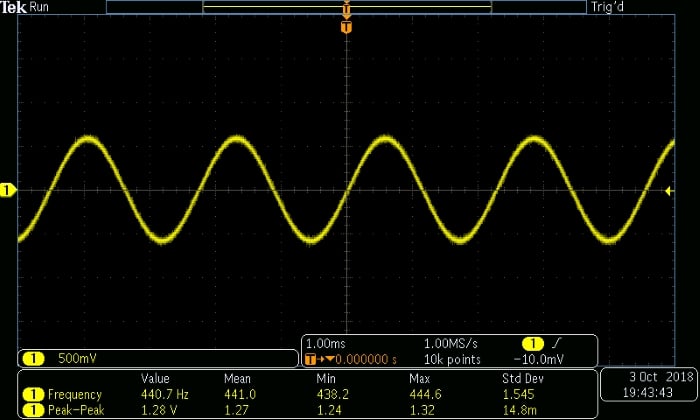
Volume setting: 50%

 

Volume setting: 80%

Generating a Triangle Wave

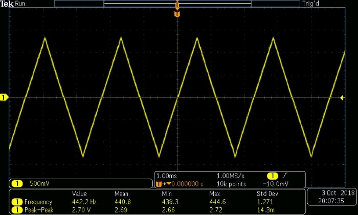
The following commands can be used to generate a triangular waveform. We’ll use the same frequency (i.e., 441 Hz), which means that the upward ramp and the downward ramp must have a length of 25 samples.

 

LowerLimit = -1;
UpperLimit = 1;
StepSize = (UpperLimit - LowerLimit)/(length(n)/2);
UpwardRamp = LowerLimit:StepSize:(UpperLimit - StepSize);
DownwardRamp = UpperLimit:-StepSize:(LowerLimit + StepSize);
TriangleWave_OneCycle = [UpwardRamp DownwardRamp];
TriangleWave_Full = -1;
for k=1:(10/CycleDuration)
  > TriangleWave_Full = [TriangleWave_Full TriangleWave_OneCycle];
  > end
sound(TriangleWave_Full)

 

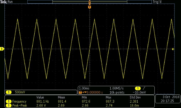
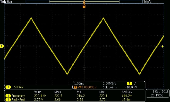
Before we finish up, I want to point out that this setup provides not only convenient amplitude control but also quick frequency adjustments: you can change the frequency of the analog waveform, without modifying the numerical values, by specifying a different sampling frequency when you call the sound() function. For example, if the specified sampling frequency is higher than the original frequency by a factor of 2, the new waveform frequency will be higher than the original waveform frequency by a factor of 2.

 

sound(TriangleWave_Full, SamplingFrequency*2)

 

sound(TriangleWave_Full, SamplingFrequency/2)

 

Conclusion

We’ve discussed a straightforward technique that uses Scilab (or MATLAB) to turn an ordinary computer into an arbitrary waveform generator. This article provides Scilab commands for generating a sinusoid and a triangle wave, and we’ll look at other waveform types in the next article.