Facebook
 Google
 GitHub
 Linkedin
Frequency Analysis: the Fast and Continuous Fourier Transforms
Jean Fourier was a mathematician who was active in the French Revolution. He was arrested twice in the fight between the various factions but was spared the guillotine. In 1798, he joined Napoleon's army in the invasion of Egypt. He was then appointed prefect in Grenoble. In 1809, Napoleon made him a baron.
In between his political and administrative duties, Fourier found time to not only publish a massive work on ancient Egypt but also to do mathematical research. He analyzed the flow of heat in mathematical terms, coming up with a novel expansion of functions as trigonometrical series. His memoir, On the Propagation of Heat in Solid Bodies, was read to the Paris Institute in 1807.
His method, now called the Fourier series, was criticized by the leading French mathematicians. It wasn’t published until 1822, and it wasn’t translated into English until 54 years later. It turned out to have applications in a wide range of areas, eventually including electronics.
The Fast Fourier Transform
When a sine wave is distorted, it creates other, higher frequencies. These frequencies can be extracted in a Fourier series. There is an algorithm called the fast Fourier transform (FFT) that does this with fewer computations compared to the original discrete Fourier transform.
Consider the sine wave in Figure 7-2, for example.

Figure 7-2. Distorted sine wave.
Here, the positive half of a 5 kHz sine wave has been compressed. Below, in Figure 7-3, it’s converted into a frequency spectrum with the help of a fast Fourier transform.
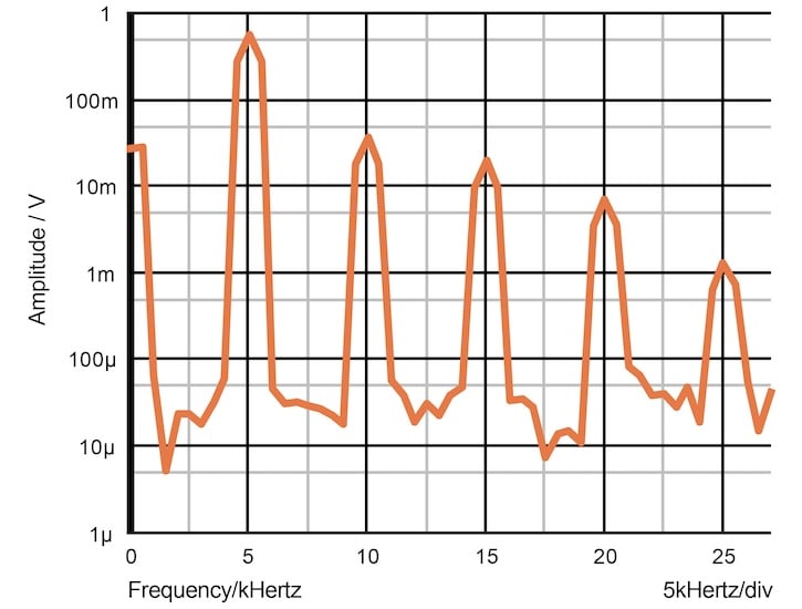
Figure 7-3. Fast Fourier transform with low resolution.
In the figure above, the peak at 0 kHz shows the DC level (the asymmetry caused by the clipping). We also see peaks at the fundamental frequency of 5 kHz and a series of harmonics:
- 10 kHz (second harmonic).
- 15 kHz (third harmonic).
- 20 kHz (fourth harmonic).
- 25 kHz (fifth harmonic).
The harmonics continue after this point with gradually decreasing amplitudes, but you can usually disregard harmonics after the fourth or fifth because their amplitudes are so small.
The amount of distortion is the square root of the sum of the squares of all harmonics divided by the amplitude of the fundamental:
$$\text{Harmonics} ~=~ \sqrt {(36~\text{mV})^2 ~+~ (21~\text{mV})^2 ~+~ (8.2~\text{mV})^2 ~+~ (0.9~\text{mV})^2} ~=~ 42.5 ~\text{mV}$$
$$\text{Fundamental} ~=~ 550~\text{mV}$$
$$\text{Distortion} ~=~\frac{\text{Harmonics}}{\text{Fundamental}}~=~ \frac{42.5}{550} ~=~ 0.077 ~=~ 7.7 \%$$
Running a Fast Fourier Transform in SPICE
Before you run a fast Fourier transform in SPICE, you need to choose two settings:
- How many samples will be taken over one period of the waveform.
- How many periods will be analyzed.
In the example we just examined (Figure 7-3), there are, in fact, too few samples and periods. This results in broad peaks.
As a general rule, start with a minimum of 25 samples and 50 periods. The number of samples is determined in the simulation by the maximum timestep and maximum print step. For our next example, we’ll use a 5 kHz driving frequency. We should, therefore, set these maximums to 8 μs:
$$Timestep~=~\frac{1}{f}~\times~\frac{1}{25}~=~\frac{1}{5000}~\times~\frac{1}{25}~=~8~\mu \text{s}$$
The number of periods is determined by the total time in the transient analysis (1 ms for 50 periods at 5 kHz). You’ll get the best results if both the number of samples per period and the number of periods are integers.
The fast Fourier transform has some flaws and limitations. For example, Figure 7-4 (our 5 kHz simulation) shows peaks in between the harmonics that, in reality, aren’t there.

Figure 7-4. Fast Fourier transform showing false peaks because of still-insufficient resolution.
The Continuous Fourier Transform
A superior method is the continuous Fourier transform, available in some analysis programs and shown in Figure 7-5.
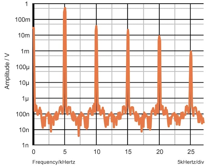
Figure 7-5. Continuous Fourier transform with high resolution.
Analyzing Triangular Waves
When you have a symmetrical waveform that isn’t a sine wave, you get only odd harmonics (third, fifth, seventh, etc.). For example, Figure 7-6 shows a triangular wave. Total distortion—the deviation from a sine wave—is 12%.

Figure 7-6. Triangle wave.
In Figure 7-7, we see the frequency spectrum of this wave.

Figure 7-7. Fourier analysis of a triangle wave.
When you have nonlinearity in a circuit and two frequencies are present, it creates differences as well as harmonics. This is known as intermodulation distortion.