How Pulse Duration Shapes Distortion and Recovery in Flat-Top PAM

As the simplest type of pulse modulation, PAM operates as a linear method in which the amplitude of each transmitted pulse is directly determined by a sample of the continuous message signal. In flat-top PAM implementations, distortion known as the aperture effect attenuates higher frequencies of the recovered message signal, which may necessitate equalization for faithful signal recovery.

In this article, we’ll first examine the aperture effect and equalization technique in flat-top PAM. Then, we’ll learn how PAM demodulators can employ a sample-and-hold circuit to enhance the recovered signal amplitude. Toward the end of the article, we’ll briefly learn about intersymbol interference (ISI) in PAM systems.

 

Overview of Flat‑Top PAM Fundamentals

Flat‑top PAM produces a train of pulses whose amplitudes follow the sampled values of the message signal. Figure 1 illustrates a representative message signal alongside its corresponding flat‑top PAM waveform.

 

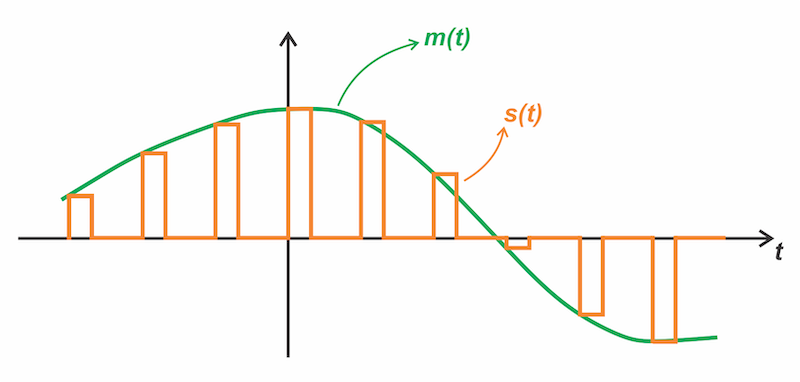
Figure 1. Message signal (green) and the corresponding PAM waveform (orange).

 

To obtain a time‑domain expression for the PAM waveform, we define a unit‑amplitude pulse p(t) centered at the origin, as illustrated in Figure 2.

 

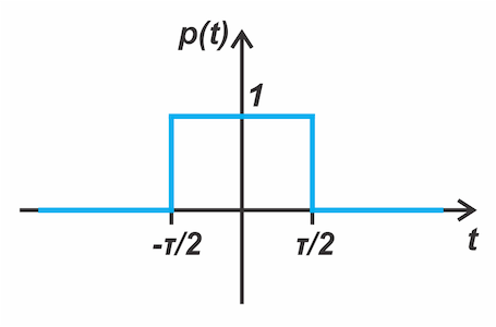
Figure 2. Unit‑amplitude pulse p(t) centered at the origin.

 

Then we can show that the PAM waveform may be written as the convolution of p(t) with a summation term, as given below:

$$s(t) = p(t) * \underbrace{\sum_{n=-\infty}^{\infty} m\! \left(nT_s \right) \, \delta(t - nT_s)}_{m_s(t)}$$

Equation 1.

where:

T_s is the sampling period

m(nT_s) denotes the value of m(t) sampled at time t = nT_s

The summation term, denoted by m_s(t), is simply an impulse train weighted by the sample values. Representing the PAM waveform using Equation 1 streamlines spectral analysis because convolution in the time domain corresponds to multiplication in the frequency domain. These functions have well‑known Fourier transforms. The Fourier transform of p(t) is a sinc function:

$$P(f) = \tau\,\mathrm{sinc}(\pi f \tau)$$

Equation 2.

where:

sinc(x) = sin x / x

τ is the pulse duration

The Fourier transform of a message signal multiplied by an impulse train consists of shifted replicas of the message spectrum, repeated at integer multiples of the sampling frequency.

 

Visualizing PAM Spectra With a Flat Message

For illustration, let’s take m(t) to have a flat spectrum extending from DC up to fm, as shown in the top sub‑figure of Figure 3.

 

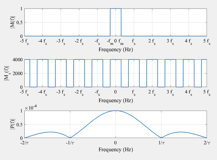
Figure 3. Magnitudes of the Fourier transforms of the message m(t) (top), its instantaneously sampled version m_s(t) (middle), and the unit‑amplitude pulse p(t) (bottom).

 

The spectrum of the instantaneously sampled signal m_s(t) comprises replicas of the original message spectrum, as illustrated in the middle sub‑figure. The bottom sub-figure shows the spectrum of p(t) for a pulse duration of τ = 100 ms. Note that the sinc function crosses zero at frequencies f = ±k / τ for all non-zero integers k. Multiplying M_s(f) with P(f) produces the spectrum of the modulated signal s(t), as shown in Figure 4.

 

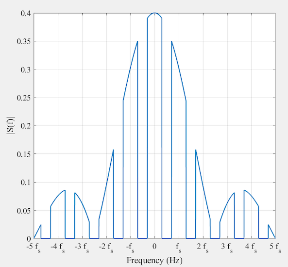
Figure 4. The spectrum of the flat-top PAM signal.

 

Figure 5 provides a closer view of the flat‑top PAM spectrum, focusing on the frequency range below f_s / 2.

 

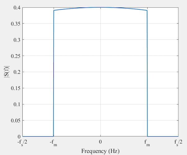
Figure 5. Zoomed‑in view of the flat‑top PAM spectrum, showing the frequency components below f_s/2.

 

As observed, a replica of the message spectrum appears in the baseband region. However, the higher frequencies of the spectrum experience greater attenuation relative to those near DC. It is clear that the receiver can readily recover the message by applying a low‑pass filter with appropriate cut-off frequency to isolate the baseband component, provided the distortion is not severe.

 

Distortion in PAM Systems Due to Aperture Effect

Flat‑top sampling can be viewed as passing the sampled signal m_s(t) through a system with transfer function P(f). Since P(f) rolls off at high frequencies, it acts as a low‑pass filter that suppresses the upper portion of the message spectrum. This distortion arises because the message m(t) is observed through a finite, rather than infinitesimal, time aperture, and is therefore termed aperture effect distortion.

The key question is how to reduce this distortion. The first spectral null of P(f) occurs at 1 / τ. When this null lies far beyond the maximum message frequency f_m, the sinc‑shaped spectrum is nearly flat across the message bandwidth, and distortion is minimal. Thus, the condition required is:

$$\tau \ll \frac{1}{f_m}$$

Equation 3.

 

As τ decreases, the distortion diminishes. In the limit τ → 0, we obtain instantaneous sampling, whose spectrum was shown in the middle sub‑figure of Figure 3, with distortion approaching zero. Therefore, flat-top PAM can be viewed as a generalization of impulse-train sampling.

 

Equalization

To limit the aperture effect distortion, the pulse duration τ should be made as small as possible. Yet, since bandwidth grows inversely with pulse duration, excessively short pulses would demand impractically large channel bandwidth. Furthermore, as will be discussed shortly, a longer pulse duration τ is beneficial because it increases the output signal amplitude. Given this trade-off, if the chosen pulse duration results in severe distortion, the receiver can apply an equalizer to mitigate it, as illustrated in Figure 6.

 

Figure 6. Block diagram for recovering m(t) from the PAM signal s(t). An equalizer is cascaded with the low‑pass reconstruction filter to mitigate the distortion.

 

In the block diagram above, the reconstruction filter is a low‑pass filter that extracts the baseband component of the flat‑top PAM signal to recover the message. If the maximum frequency in m(t) is fm, then the sampling rate fs must exceed the Nyquist rate, 2f_m. Therefore, the filter cutoff should be chosen between f_m and f_s − f_m.

The equalizer applies the inverse of the loss introduced by the pulse shape (the aperture effect). Ideally, the equalizer’s response should be:

$$H_{eq}(f) = \frac{1}{P(f)} = \frac{1}{\tau\,\mathrm{sinc}(\pi f \tau)} = \frac{\pi f}{ sin( \pi f \tau) }$$

Equation 4.

 

This lets the equalizer compensate for the high‑frequency attenuation caused by the pulse shape spectrum. Designing a filter that implements the transfer function in Equation 4 over a wide frequency range is generally difficult, especially because P(f) equals zero at certain frequencies. However, because the message signal has a limited bandwidth, the equalizer only needs to approximate 1 / P(f) within that range. In mathematical terms, we should have:

$$H_{\text{eq}}(f) =\begin{cases}\dfrac{1}{P(f)}, & |f| \leq f_m, \\0, & \text{elsewhere.}\end{cases}$$

Equation 5.

 

Equalization works because aperture-effect distortion introduces a known, predictable weighting to the signal’s spectrum. The equalization required in practical systems is generally minimal because the pulse duration is often small. When the duty cycle satisfies τ / T_s ≤ 0.1, the amplitude distortion falls below 0.5%, making equalization unnecessary in most cases.

 

Signal Recovery Through Holding

As previously discussed, recovering the message signal from a PAM waveform typically requires a lowpass filter and an equalizer. However, when the pulse duration is excessively short, we may need to employ a sample-and-hold circuit within the demodulation chain, prior to the lowpass filter. Figure 7 shows the basic sample-and-hold circuit for PAM message recovery.

 

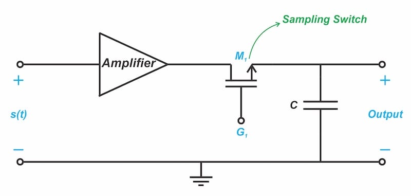
Figure 7. Signal recovery from a PAM waveform using a sample-and-hold circuit.

 

To understand the operation of the circuit above, we must first understand how the pulse duration affects the output signal amplitude. Intuitively, a shorter pulse duration τ reduces transmitted energy. This effect is quantitatively confirmed by Equations 1 and 2. Specifically, the spectrum of the sampled signal, M_s(f), consists of replicas of the message spectrum scaled by 1 / T_s (as shown in Figure 3). Since the PAM signal’s spectrum is M_s(f)P(f), the final recovered message spectrum is scaled by P(f) / T_s, which simplifies to:

$$\text{Scaling Factor} = \frac{P(f)}{T_s} = \frac{\tau}{T_s}\,\mathrm{sinc}(\pi f \tau)$$

Equation 6.

 

This shows that an excessively short pulse duration τ can result in unacceptably low amplitude in the recovered message signal. A sample-and-hold circuit mitigates this issue by extending the pulse width to increase the signal level, providing effective amplification while circumventing the noise associated with additional active gain stages. Figure 8 illustrates the pulse-width extension provided by the sample-and-hold circuit.

 

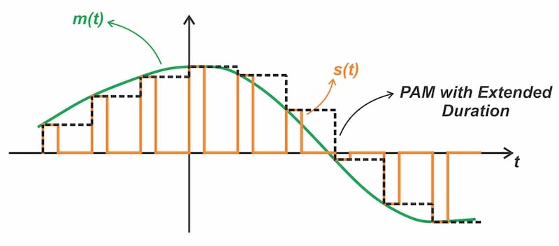
Figure 8. Pulse-width extension using a sample-and-hold circuit.

 

The waveform above holds the value of each pulse until the next pulse appears. Because the aperture effect distortion grows with pulse duration, we can also opt for a smaller increment in the pulse duration to ease equalization.

Before moving forward, note that the sample-and-hold switch in Figure 7 operates synchronously with the incoming pulse train: it closes with a short delay following the pulse leading edge and opens prior to the trailing edge. Furthermore, the amplifier preceding the sampling switch is configured as a buffer to drive the sample-and-hold circuit, and its gain is incidental to the core operation discussed here.

 

Intersymbol Interference in PAM Systems

Before we conclude, I want to highlight an important phenomenon related to transmitting pulses through communication channels. When a rectangular pulse passes through real-world filters and channels, the finite bandwidth of the system slows down the pulse transitions. As the pulse spreads out in time, some of its energy leaks beyond the intended duration. Due to this smearing effect, the decaying tail of one pulse may interfere with subsequent pulses, causing a distortion known as intersymbol interference (ISI). To understand this, consider transmission of a bit stream through a long PCB trace, as illustrated in Figure 9.

 

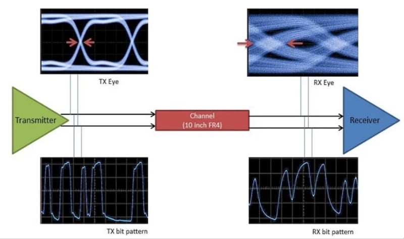
Figure 9. The effect of elongated rise/fall times on the transmission of a bit stream. Image used courtesy of TI.

 

While the signal transitions are sharp at the transmitter side, they slow down, as the signal travels to the far end of the transmission line. When several consecutive bits have the same value, the received signal can reach its final value despite the elongated rise and fall times. However, in a bit stream that alternates between 1s and 0s, like 101010101, the transmitted pulses are shorter, and the output doesn't have enough time to reach its final value. Thus, whether a transition reaches its final value depends on the bit pattern.

To mitigate this distortion, systems use pulse shaping filters to reshape the waveform, allowing it to fit within the channel’s available bandwidth while controlling ISI. Common options for minimizing ISI include raised cosine and root-raised cosine pulses. In a future article, we will explore the ISI effect in greater detail and learn more about pulse shaping.

 

Wrapping Up

While examining aperture-effect distortion in flat-top PAM and the equalization used to compensate for it, we saw how a sample-and-hold circuit can increase the recovered signal amplitude. The distortion caused by flat-top PAM when transmitting an analog, information-bearing signal is called the aperture effect. Because the aperture effect distortion introduces a known, predictable weighting to the signal’s spectrum, we can use equalization to compensate for this distortion and recover the message.

When τ / T_s ≪ 1, PAM systems require minimal, if any, equalization. Another type of distortion that occurs when transmitting pulses through band-limited communication channels is ISI, which can be mitigated using pulse shaping techniques. While this article focused on distortion in flat-top PAM, the next article will explore ISI and pulse shaping in greater detail.