How the Weibull Distribution Is Used in Reliability Engineering

This article discusses the Weibull distribution and how it is used in the field of reliability engineering.

Reliability engineering uses statistics to plan maintenance, determine the life-cycle cost, forecast failures, and determine warranty periods for products.

This is a common topic discussed across all engineering fields and often seen in power electronics, in particular. If you have to design a product for space, medicine, or other specialized fields, where subsystem failures can cause mission failure or loss of life, you should study the New Weibull Handbook, upon which this article is based.

If you spend any amount of time in reliability engineering, you will undoubtedly encounter the Weibull distribution. Swedish engineer Waloddi Weibull introduced this probability distribution to the world in 1951 and it is still in wide use today.

Before you get started, you may consider reading my first article introducing the concept of reliability engineering for some background information.

Plotting Failures—The Path to Weibull

Families of products used in a similar fashion will fail along predictable timelines. This excludes failures due to external factors (electrostatic discharge, mishandling, intentional abuse, etc.).

Weibull plots record the percentage of products that have failed over an arbitrary time-period that can be measured in cycle-starts, hours of run-time, miles-driven, et al. The time-scale should be based upon logical conditions for the product. For example, an oscilloscope might be “hours of run-time”, while a vehicle instrument cluster might be measured in “road miles” and a spring-pin programmer in “# of times used”.

The data is recorded on a log-log plot.

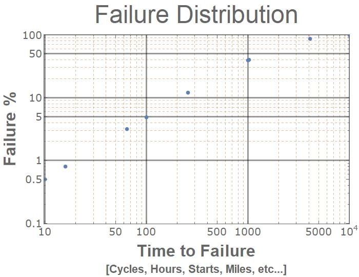
Figure 1. This time to failure graph shows the percentage of a widget that has failed over time.

The slope of the graph is not linear—but a straight, best-fit line does provide a decent approximation.

The slope of that best-fit line, β, describes the Weibull failure distribution.

• β<1.0 indicates infant mortality
• B=1 means random failure
• β>1 indicates wear-out failure.

(See chapter 2 of The New Weibull Handbook for more details.)

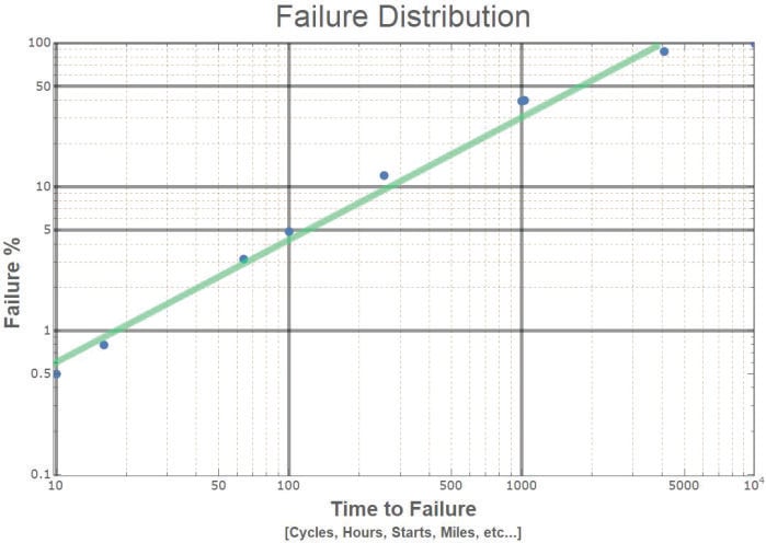
Figure 2

The time-to-failure of a particular percentage of a product is described historically as the B1, B10, B20, etc… time, where the number describes the percentage of products that have failed. For example, B10 is when 10% of the products have failed.

Some manufacturers use L-times (L1, L10, L20, etc…), where L stands for “lifetime”. Weibull distributions describe a large range of products; B is thought to possibly stand for “Bearing Life”.

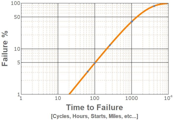
Figure 3. A Weibull CDF fitted to the sample data from the previous graph. In this instance, β=1 and η=2000.

The Weibull continuous distribution is a continuous statistical distribution described by constant parameters β and η, where β determines the shape, and η determines the scale of the distribution.

Continuous distributions show the relationship between failure percentage and time.

In Figure 3 (above), the shape β =1, and the scale η=2000. The following graphs will illustrate how changing one of these variables at a time will affect the shape of the graph.

As η changes, the Weibull plot shifts and stretches along the horizontal axis.

Figure 4. Weibull CDF plot shows changing η with β =1

As β changes, the slope and shape of the graph change as shown below in Figure 5.

Figure 5. Weibull CDF Plot shows the effect of changing β as η=2000

Additionally, some sources introduce the variable μ, that shifts the graph along the horizontal time-axis (t-μ).

The equation is unfortunately represented with different variables by different sources, α, β, η, λ, κ, etc. The convention adopted in this article models the New Weibull Handbook.

Probability Density Function

Accumulating the failures shown above over time generates a probability density function (PDF). This new equation shows how many products will fail at a particular time.

If you ran a data-center, this graph would provide useful information for determining how many spare parts to keep on hand, or for scheduling preventative maintenance.

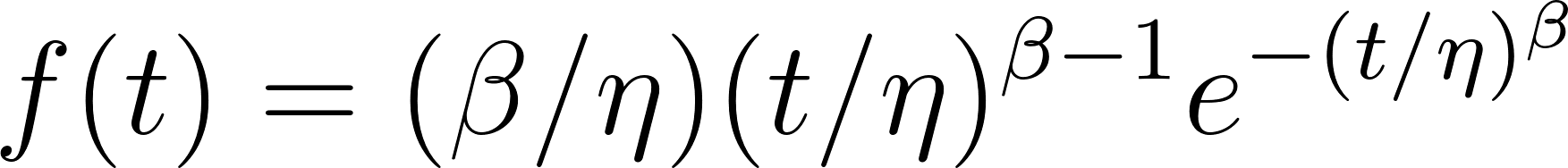
This probability density function describes the frequency of failures over time.

Two interesting things to note about the equation above:

• First, when β = 1, the equation simplifies to a simple exponential equation.
• Second, when β ≈ 3.4, the graph looks like a normal distribution, even though there is some deviation.

Figure 6

The scale parameter η equals the mean-time-to-failure (MTTF) when the slope β = 1. Discussion of what occurs when β ≠ 1 is beyond the scope of this article. Interested readers should again refer to the New Weibull Handbook or other resources online.

How are Failure Rates Determined?

If you look at failure data, you will occasionally run into MTTF times that are, well, ridiculous. For example, Linear Devices GaN HEMT wafer process technology reliability data provides an MTTF of 15,948,452,200 hours. I assure you that Linear did not begin testing their wafers 1.8 million years ago, when homo sapiens were discovering fire.

So how was this number calculated?

Manufacturers accelerate the decomposition of their products by exposing them to excessive heat and excessive voltage. These accelerated failure tests can then be used with specific equations to calculate how long a device will last.

Imagine placing a bar of chocolate directly above a campfire. The closer the chocolate is to the fire, the more heat energy is transferred to it and the quicker it melts. But if the chocolate bar stays a suitable distance away, it will never melt and will last virtually forever.

Temperature Acceleration

Temperature acceleration exposes devices to high temperatures—125 °C, 150 °C, and beyond—and relates the use temperature MTTF to the test temperature MTTF using the Arrhenius equation.

Where t_test and t_use are the MTTF, k is Boltzmann’s constant

and E_a is the activation energy for a specific failure mechanism. Linear Technology’s Reliability Handbook provides the value of 0.8 eV for failure due to oxidation and silicon junction defects, and 1.4 eV due to contamination.

Voltage Acceleration

Sometimes manufacturers will expose their devices to excessive voltage. There, an acceleration factor is calculated with a different equation.

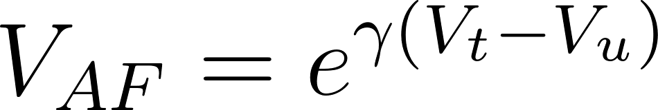
Where γ is the voltage acceleration constant that is “derived from time-dependent dielectric breakdown testing”, and V_t & V_u are the test and use voltages.

Highly Accelerated Stress Testing

When manufacturers are really in a rush to find failures, they can subject their devices to high-pressure, high-humidity, high-temperature environments for prescribed periods of time. They can perform rapid and extreme temperature cycling, expose their devices to electromagnetic energy, vibration, shock, and other factors.

All of these tests can then be mathematically interpreted to provide actual MTTFs that reliability engineers can then use in their calculations.

Summary

Reliability engineers use statistics and mathematical analysis to predict how long their devices will function. By knowing how long a device should work, they can predict warranty periods, plan preventative maintenance, and order replacement parts before they are needed.

This is just a brief introduction to the field. If you are a reliability engineer and know of other sources of information, please let us know about them in the comments below!