 Facebook
 Google
 GitHub
 Linkedin
How to Interpret IMU Sensor Data for Dead-Reckoning: Rotation Matrix Creation
Working with IMUs can maddening for a variety of reasons, but what scares people the most is usually the math.
Working with IMUs can maddening for a variety of reasons, but what scares people the most is usually the math.
IMU data is useless unless you know how to interpret it.
For example, the BNO055 is a 9DOF sensor that can provide acceleration, gyroscopic, and magnetometer data, as well as fused quaternion data that indicates absolute orientation from an initial position. All of that data is completely useless unless you can find a way to relate the IMU’s frame of reference to a fixed, external reference frame.
Data from uncalibrated sensors are useless.
And once you figure out how to stabilize the data in an inertial reference frame, misaligned axes can still wreak havoc on all of your hard work. If you are not careful, you will end up making calculations with data that is mixed among multiple axes of movement.
A calibrated sensor still needs to be aligned with an inertial reference to make the data truly useful.
You usually have to align your sensor with your inertial reference frame to be able to interpret the data.
Once your sensor is aligned in the inertial frame, you can align your data.
The way to do this is with rotation matrices whose individual elements are populated with trigonometric functions or quaternions. Quaternions are preferred because they require less computation by an MCU.
In this article, I will describe a rotation matrix and present some of the mathematics required to configure the Bosch BNO055 IMU for the purposes of dead-reckoning. I am using this IMU because I have one on hand from a previous article on how to capture data with the BNO055.
Interested readers might like to know that Bosch replaced this IMU with the BMX055. However, the mathematics presented here should work with any sensor system. The focus of the article is on the mathematics, not the sensor.
Whichever sensor you use, you must calibrate the device according to the manufacturer's datasheet prior to every use. Sometimes that calibration requires an external EEPROM.
Rotation Matrices
Moving a vector around in three-dimensional space can be a complicated affair. One common technique uses sequential rotations around fixed axes to rotate vectors.
The easiest way to reorient your vectors in a single rotation is with a rotation matrix. A 3×3 matrix contains all of the necessary information to move a vector in a single rotation without using trigonometry.
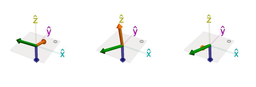
The above gravity vectors (orange) are rotated about a single axis (green) to lie in the negative z-axis (blue)
You can learn more about that technique by searching for “Euler angles” or by reading my previous article on quaternions.
In the gifs below, you can see sequential rotations for yaw, pitch, and roll, each of which requires a specific orientation of axes for proper function. Whenever a single movement can be described by multiple rotations, gimbal-lock is possible.
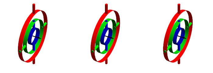
Rotations for yaw, pitch, and roll
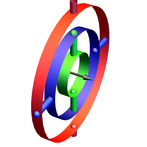
Roll, pitch, and yaw rotations are popular, but ultimately mathematically flawed.
The trouble with using roll, pitch, and yaw is that it is cumbersome, utilizes trigonometry and is subject to gimbal lock. Trigonometric functions require hundreds of clock cycles in a microprocessor that can negatively affect the performance of your code. Whenever possible, code should use simpler mathematical functions.
A three-dimensional vector that lies on the unit sphere can be rotated into any new position with a single rotation about a fixed axis. It is much faster and only requires the basic calculations of add, subtract, divide, and multiply.
However, it does require you to do some math before you begin to program.
Example Orientation Configuration: Bosch BNO055
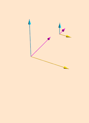
So here’s the scenario that we’ll be working through. The BNO055 is inside a soccer ball, it’s turned on, data is written from EEPROM memory to the calibration registers, and the device is sitting somewhere in a room. We don’t really know what the orientation is, so any data we take off of the device could be pointing in any direction.
We will create a rotation matrix that aligns the sensor data such that the force of gravity points in the direction of the negative z-axis. Later, we can align the magnetic north to lie along the x-axis.
The BNO055 outputs a gravity vector. As shown in the graphic below, the gravity vector always points down. We will find the matrix required to mathematically rotate the sensor so that the gravity vector lies along the negative z-axis.
A rendering of a gravity vector. The animated circles represent the direction of positive rotation that corresponds to the right-hand rule
As a note, if the sensor didn't output a gravity vector, we could simply read data from the three axes of the accelerometer and perform similar steps. We would, however, have to be a bit more careful with variable assignment.
Gravity Vector Code
The following code reads the gravity vector from the BNO055
#include <Wire.h>
#include <Adafruit_Sensor.h>
#include <Adafruit_BNO055.h>
#include <utility/imumaths.h>
/*
This program is an abridged version of Adafruit BNO055 rawdata.ino available after installing the Adafruit BNO055 library. Program modified by Mark Hughes for AllAboutCircuits.com
File→Examples→Adafruit BNO055→Raw Data
Connections on Arduino Uno
=========================================================================
SCL to analog 5 | SDA to analog 4 | VDD to 3.3V DC | GND to common ground
*/
#define BNO055_SAMPLERATE_DELAY_MS (100) // Delay between data requests
Adafruit_BNO055 bno = Adafruit_BNO055(); // Create sensor object bno based on Adafruit_BNO055 library
void setup(void){
Serial.begin(115200); // Begin serial port communication
if(!bno.begin()) // Initialize sensor communication
{
Serial.print("Ooops, no BNO055 detected ... Check your wiring or I2C ADDR!");
}
delay(1000);
bno.setExtCrystalUse(true); // Use the crystal on the development board
}
void loop(void)
{
imu::Vector<3> gravity = bno.getVector(Adafruit_BNO055::VECTOR_GRAVITY);
Serial.print("gX: ");Serial.print(gravity.x()); Serial.print("\t");
Serial.print("gY: ");Serial.print(gravity.y()); Serial.print("\t");
Serial.print("gZ: ");Serial.print(gravity.z()); Serial.print("\t");
Serial.println("");
}
------ Output -------
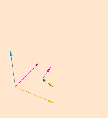
gX: 0.59 gY: 9.15 gZ: -3.47The acceleration due to gravity near the surface of the Earth is approximately 9.801 m/s². That the sensor reads 9.15 in the Y direction indicates that the sensor is tipped nearly on end (as shown below). Our goal is to make the X and Y components of gravity 0 and the Z component of gravity nearly 9.8.
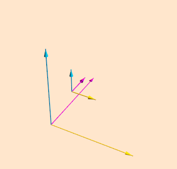
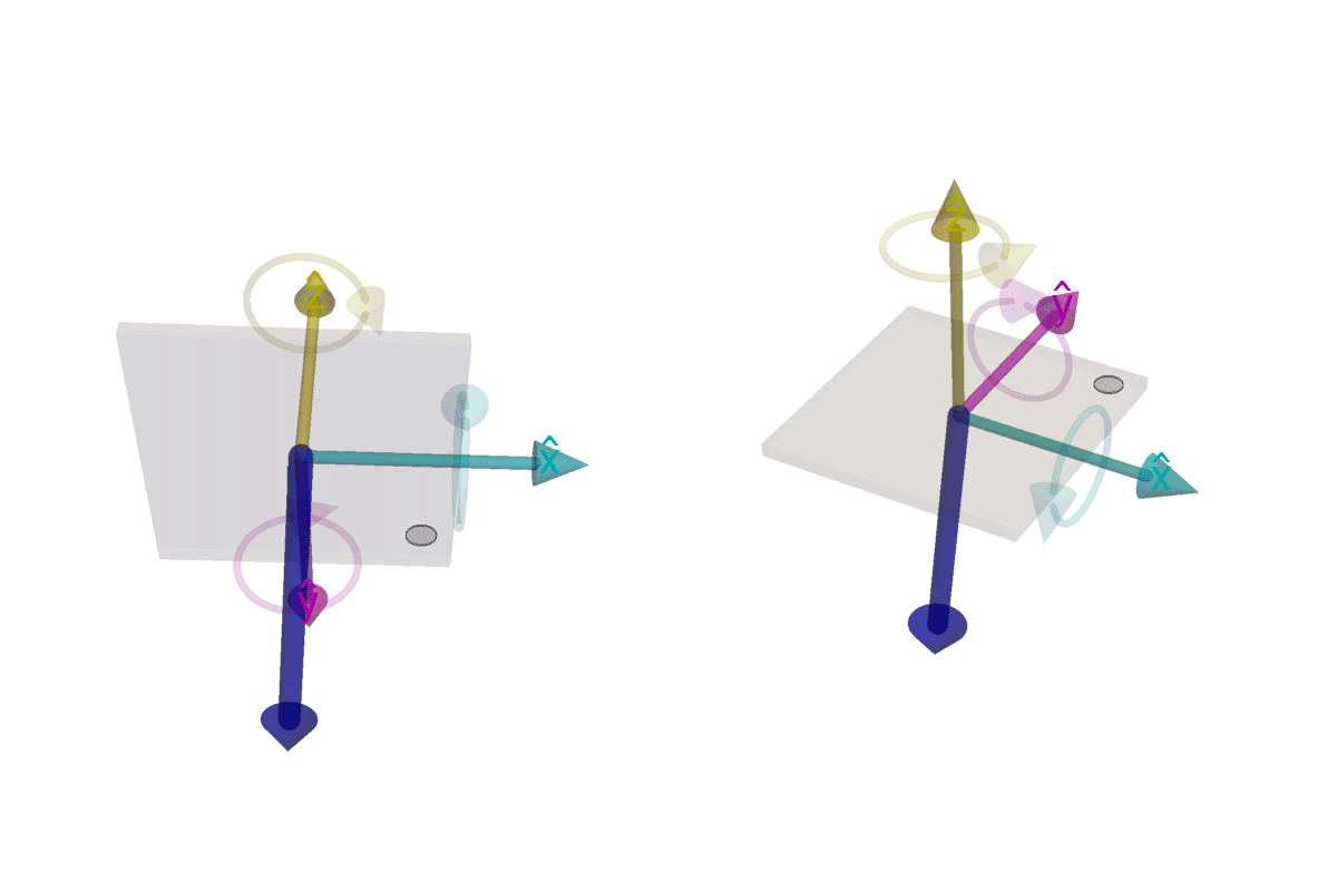
Below you can see a rendering of sensor orientation, represented by the dark blue pointer. On the right is the orientation at startup. On the left is the orientation that is closer to the ideal, with the negative z-axis parallel to the gravity vector.
Left: Sensor orientation at startup. Right: Closer to the ideal sensor orientation.
Determining the rotation matrix needed to rotate the sensor into the proper position requires some mathematics. First, the vector coming out of the sensor and our target vector must be normalized. This is necessary to make the equations solvable. Without normalization the terms become quite unwieldy, involving imaginary terms and conjugates. On my machine, it came out to approximately 4 pages of size 14 font.
Normalization gives a vector that has only direction—the length of a normalized vector is one. To normalize, divide each component by the square root of the sum of the squares of each component. An example, made from actual sensor data, is shown below.
$$\hat{A}= \left \{\frac{A_x}{\sqrt{A_x^2+A_y^2+A_z^2}}\;\hat{x}, \frac{A_y}{\sqrt{A_x^2+A_y^2+A_z^2}} \; \hat{y} , \frac{A_z}{\sqrt{A_x^2+A_y^2+A_z^2}} \;\hat{z} \right \}%0$$
$$\hat{A}= \left \{\frac{0.59}{\sqrt{0.59^2+9.15^2+(-3.47)^2}}\;\hat{x}, \frac{9.15}{\sqrt{0.59^2+9.15^2+(-3.47)^2}} \; \hat{y} , \frac{-3.47}{\sqrt{0.59^2+9.15^2+(-3.47)^2}} \;\hat{z} \right \}$$
$$\hat{A}= \left \{0.061\;\hat{x}, 0.933 \; \hat{y} , -0.354 \;\hat{z} \right \}$$
Since we chose the target vector as being the negative z-axis, we don’t have to go through the trouble of normalizing it.
$$\hat{G}=\left\{ 0\; \hat{x}, 0\; \hat{y} , -1 \;\hat{z}\right\}%0$$
Vector Mathematics
Dot Product
To determine the part of vector A that is projected onto vector G, use the dot product.
$$\hat{A}\cdot \hat{G}=\left | A \right | \left | G \right |cos(\theta)$$
And to find the angle between them, rearrange the equations to solve for θ.
$$cos(\theta)=\frac{\hat{A}\cdot \hat{G}}{\left | A \right | \left | G \right |}$$
Our vector normalization is already paying off. Since |A| and |G| are both already set to one, the denominator disappears. Additionally, since the X and Y components of G are zero, the equation reduces rapidly.
$$cos(\theta)=A_x\cdot 0+A_y\cdot 0\;+\;-1\cdot A_z$$
So the angle of rotation depends only on the Z component of the acceleration.
$$\theta=arccos(-1\cdot A_z)$$
Cross Product
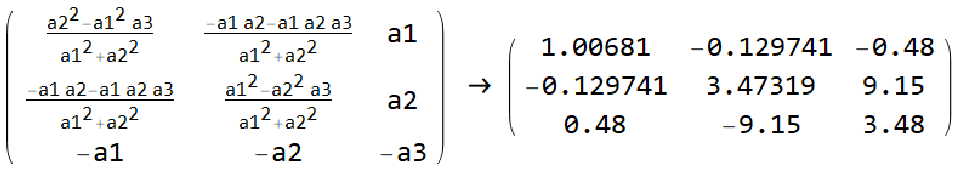
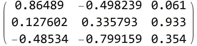
Determining the vector to rotate this angle around is not for the faint of heart. Not that it’s particularly difficult, but it is particularly tedious. There are several steps, and it is easy to make a little mistake. This is where programs such as Mathematica shine—they don’t make mistakes unless their human programmers tell them to. Below is the rotation matrix before I told the program that I was using unit vectors
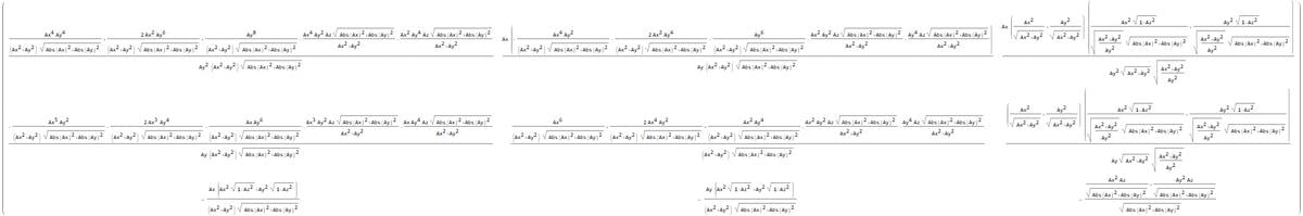
Once you realize that there are several simplifications that can be made to the matrix, it reduces quickly to something far more manageable
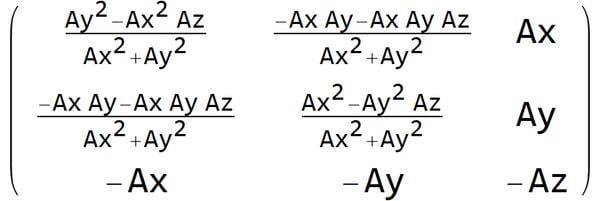
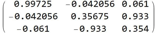
And after the substitution of our original values, we have a rotation matrix that will rotate our gravity vector into the negative z-axis. And there are certain symmetries that can be taken advantage of to further reduce computational complexity.
This matrix, based on the gravity vector, is determined once at start-up to get an orientation with respect to gravity. If applied to future acceleration readings, this matrix will rotate the values so that no matter how your sensor is mounted, the negative z-axis will point straight down. This rotation matrix, when multiplied by any acceleration vector (normalized or not), will rotate it. Let’s look at an example—and use the original gravity vector.
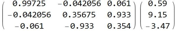
For those of you that require a brief refresher on matrix multiplication, the elements of each row of the matrix are multiplied by each element in the column. The results are totaled after rearranging the components.

When all is said and done, the result is the following:

Not exactly zero in the X direction and the Y direction—but close enough. Remember that we used only two decimal places of precision when starting this journey, and we have a zero reading out to two decimal places in X and Y as well as the expected -9.801 m/s². I’ll call that a win.
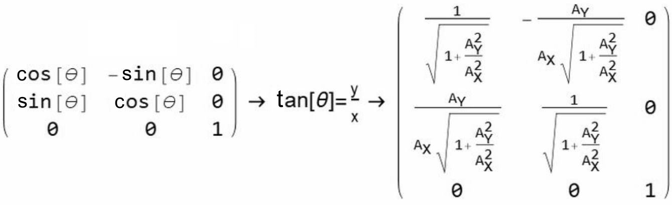
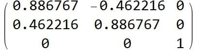
Fortunately, rotating the compass reading so that the x- or y-axis lies along magnetic north is much simpler, as the measurement values can now be rotated around the z-axis. And there is plenty of room for code simplification—temporary variables can be used to store common terms to accelerate code execution. Additionally, symmetry can be used to reduce redundant calculation.
Substituting the value of tangent of θ=Y/X into the matrix provides the rotation. You can align to the positive x-axis, the positive y-axis, the negative y-axis, or the negative x-axis by manipulating the right side of this equation (e.g., tan[θ] = -X/Y), or you can align to another angle (e.g., geographic north) by manipulating the left side of the equation (tan[θ+14°]=Y/X).
Summary
IMUs need to be calibrated in the environment in which they will operate. Part of that calibration usually requires the user to define how the sensor is oriented in space and in reference to the environment the sensor is in. This article demonstrated how to create an arbitrary rotation matrix aligned with accelerometer data as well as a two-dimensional rotation matrix based on magnetometer data.
The combined gravity and magnetometer rotation matrix transform is shown above.
The initial matrices (gravity and magnetometer) can be multiplied to create a single rotation matrix that is applied to all future measurements—ensuring that the data you collect can be successfully analyzed later.


Has anyone had success with a device like this in directional control of a relatively slow-moving, small vehicle?