How to Use Nyquist Plots for Stability Analysis

In this article, we’ll see that a Nyquist plot provides a straightforward means of determining if an amplifier will oscillate.

Supporting Information

• Negative Feedback, Part 4: Introduction to Stability
• Negative Feedback, Part 5: Gain Margin and Phase Margin
• Phase Margin Estimation Using the Rate-of-Closure

In the three preceding articles in this series, we explored the general concept of a Nyquist plot, the location of the cutoff frequency in a first-order Nyquist curve, and important characteristics of second-order Nyquist curves. Now we’re ready to introduce the primary practical application of Nyquist plots: stability analysis.

This article will briefly review essential information regarding amplifier stability, but if this subject matter is new to you (or if you need a refresher), refer to the articles listed above in the “Supporting Information” section.

 

Understanding Stability Analysis

The issue of stability figures prominently in discussions of op-amp circuits (and other negative-feedback amplifiers) because phase shift can cause negative feedback to become positive feedback, and positive feedback can cause a small input signal to increase in amplitude until the circuit becomes nonfunctional. A stable amplifier is not susceptible to saturation or oscillation induced by unintentional positive feedback.

A feedback system is characterized by an open-loop frequency response (A), a closed-loop frequency response (G_CL), and a feedback factor (β). We typically use Bode plots to represent the open-loop and closed-loop response, and a Bode plot is also handy when we need to represent the behavior of a frequency-dependent feedback network (if the feedback network is purely resistive, β is simply a number).

The critical quantity in feedback analysis is not A or β or G_CL. Rather, it is the loop gain, i.e., the frequency response experienced by a signal as it travels around the system’s loop. The loop gain is equal to Aβ, i.e., the open-loop gain multiplied by the feedback factor.

 

How to Design a Stable Amplifier

Loop gain, like open-loop gain, originates from a frequency-dependent network that produces phase shift and exhibits variations in magnitude response. An amplifier with three or more poles will have a loop gain that eventually produces more than 180° of phase shift; the frequency at which the input signal experiences 180° of phase shift is denoted by f₁₈₀. The fundamental stability criterion is that the magnitude of the loop gain must be less than unity at f₁₈₀.

 

 

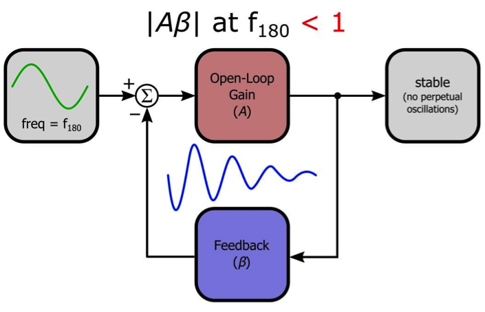
However, to ensure robust stability and desirable circuit performance, the gain at f₁₈₀ should be significantly less than unity.

Stability in the Nyquist Plot

It turns out that a Nyquist plot provides concise, straightforward visualization of essential stability information. Let’s look at an example:

 

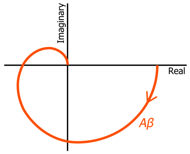
Note that I usually don’t include negative frequencies in my Nyquist plots.

 

Keep in mind that the plotted quantity is Aβ, i.e., the loop gain. We don’t analyze stability by plotting the open-loop gain or the closed-loop gain.

As explained above, the critical factor in amplifier stability is the magnitude of the loop gain at f₁₈₀. As we saw in the two preceding articles, a Nyquist plot doesn’t give us a specific numerical frequency, but it does clearly indicate the “location” of certain important frequencies, and then this location gives us relevant information about the circuit’s magnitude and phase response. In the Nyquist plot shown above, f₁₈₀ corresponds to the point at which the curve crosses the negative real axis.

 

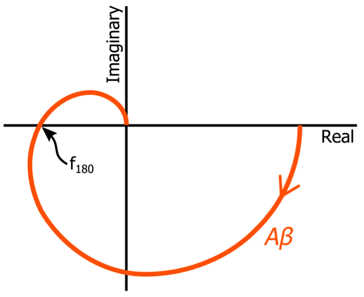
We can’t use the Nyquist plot to determine the numerical value of f₁₈₀, but in the context of basic stability evaluation, that doesn’t matter. All we need to know is the magnitude and phase at f₁₈₀, and this is exactly what the Nyquist plot provides.

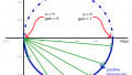
In fact, if we label the point (–1, 0)—i.e., negative one on the real axis, which corresponds to a magnitude response of unity at a phase shift of 180°—we can immediately assess the amplifier with respect to the fundamental stability criterion. Consider the following two variations on the Nyquist diagram shown above:

 

 

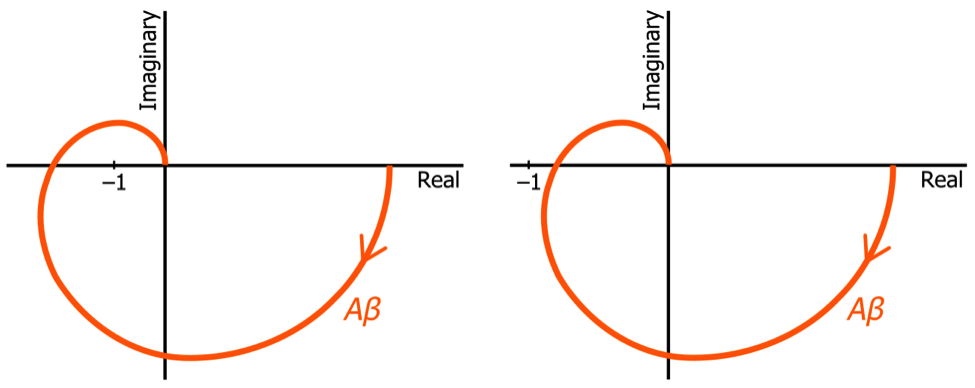
One of these plots represents a stable amplifier, and the other represents an unstable amplifier. Which is which? Well, all we need to do is calculate (or estimate) the magnitude of the Nyquist curve where it crosses the negative real axis. If the curve crosses the negative real axis to the left of (–1, 0), the magnitude of the loop gain at f₁₈₀ is greater than unity; if it crosses the axis to the right of (–1, 0), the magnitude at f₁₈₀ is less than unity. Thus, the plot on the left represents an unstable amplifier, and the plot on the right represents a stable amplifier.

In practice, we need to know not only whether the circuit is stable (according to the theoretical criterion) but also the “amount” of stability. With a Nyquist plot, you can simply observe the distance between (–1, 0) and the point at which the curve crosses the negative real axis. More distance between these two points corresponds to a larger gain margin and, consequently, to a circuit that is more reliably stable.

 

Conclusion

I hope that this article has helped you to understand why the Nyquist plot is a direct and visually simple way of conveying a circuit’s stability characteristics. In the next article, I will show you how to generate Nyquist curves in LTspice.