Facebook
 Google
 GitHub
 Linkedin
Understanding Nyquist Plots for Second-Order Filters
This article continues a series on Nyquist diagrams by explaining Nyquist curves that represent the transfer function of a two-pole filter.
This article continues a series on Nyquist diagrams by explaining Nyquist curves that represent the transfer function of a two-pole filter.
In previous articles, I introduced the Nyquist plot and then we explored these types of plots in more detail by examining the relationship between Nyquist curves and cutoff frequency with respect to first-order passive filters. In this article, we will look at Nyquist plots for second-order filters.
Review: Second-Order Filters
When I say “second-order” filter, I am referring to filters that use inductor-capacitor (LC) resonance or an amplifier to generate a true second-order transfer function. You can achieve two-pole frequency response by cascading two first-order passive filters, but the resulting circuit does not have complex-conjugate poles, and consequently, the transfer function cannot be optimized because the Q factor is always 0.5. In contrast, the Q factor of a resonance- or amplifier-based second-order filter can be controlled by the designer in such a way as to favor flat passband, linear phase response, or rapid passband-to-stopband transition.
The information in this article applies to second-order filters in general, but as I was writing the article, the circuit that I had in mind was the RLC second-order low-pass filter shown below.
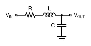
The cutoff frequency of this filter is determined by the value of the capacitor and the inductor, and the Q factor can be varied by changing the value of the resistor. When you’re working with Nyquist plots, it’s important to remember that the cutoff frequency (ωO) of a second-order filter is not necessarily the –3 dB frequency. The gain at ωO can be –3 dB, lower than –3 dB, or greater than –3 dB depending on the filter’s Q factor.
Quadrants in the Nyquist Plot
The first thing that you might notice about a second-order Nyquist plot is that it extends into the bottom-left quadrant of the complex plane. For example:
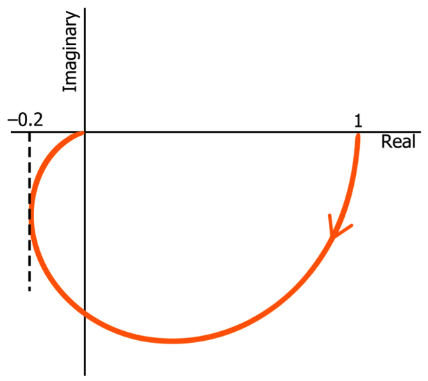
Note that all of the plots shown in this article do not include negative frequencies.
Since the curve extends into the bottom-left quadrant but not into the top-left quadrant, we know immediately that it represents a second-order filter. Why? Well, the negative imaginary axis corresponds to phase shift of –90°, and if the Nyquist trace crosses this axis and extends into the bottom-left quadrant, the filter must have more than one pole, because you only get –90° of phase shift per pole. It can’t have three poles because the angle doesn’t go past –180° (which corresponds to the negative real axis).
You can see that the curve tends toward –180° as it approaches the origin, just as the phase shift of a two-pole filter asymptotically approaches –180° as frequency increases toward infinity.
Cutoff Frequency in Second-Order Filters
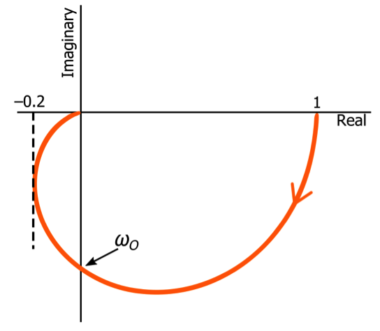
As with first-order Nyquist plots, the Nyquist plot for a second-order filter doesn’t give us a numerical cutoff frequency. In contrast to the first-order case, however, we cannot find the generic cutoff-frequency location by looking for a point on the curve with a magnitude response of $$\frac{1}{\sqrt{2}}$$, because (as mentioned above) the gain at ωO is influenced by the circuit’s Q factor.
Phase shift, however, will consistently be –90° at the cutoff frequency, regardless of Q. Thus, for a second-order low-pass filter, the cutoff frequency corresponds to the point at which the Nyquist curve crosses the negative imaginary axis.
Q Factor in Second-Order Nyquist Diagrams
Even basic Nyquist plots such as those shown above can give us important qualitative information about the Q factor of a second-order filter. If we know that we’re dealing with a passive low-pass filter, then we can assume that the low-frequency gain will be unity. Thus, the Nyquist curve will begin with a magnitude response of 1, and since the phase shift is essentially zero at very low frequencies, the Nyquist trace originates from a value of 1 on the positive real axis.
The behavior of the curve after it departs from the real axis gives us information about the magnitude response as frequency increases, and this, in turn, gives us information about Q. First of all, if the distance from the origin increases beyond the initial value, the filter’s gain increases as the input frequency approaches the cutoff frequency, and therefore Q must be high enough to cause some peaking.
Furthermore, you can form a general idea of the magnitude response in the cutoff-frequency region by comparing the gain at the cutoff frequency to the initial gain. If the cutoff-frequency gain is significantly higher than the low-frequency gain, you know that the filter has a relatively high Q.
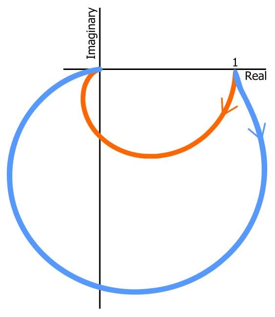
The next plot shows two Nyquist curves for RLC filters with the same cutoff frequency but different Q. The orange curve represents a critically damped filter—i.e., Q = 0.5 and the gain at ωO is –6 dB. The blue curve represents an underdamped filter; its Q factor is approximately 1.7, and the gain at ωO is +4.7 dB.
Conclusion
We’ve seen that the Nyquist plot for a low-pass filter gives us clear, direct information about the number of poles in the transfer function, and we explored the relationship between the general shape of a Nyquist curve and the Q factor of a second-order filter. We’ll continue our discussion of Nyquist plots in the next article.
This article is Part 3 in a series on Nyquist plots. All articles in this series are listed below in order of publication.
- How to Use a Nyquist Plot for AC Analysis
- Understanding Cutoff Frequency in a Nyquist Plot
- Understanding Nyquist Plots for Second-Order Filters
- How to Use Nyquist Plots for Stability Analysis
- LTspice for Nyquist Plot Analysis
Related Content