Facebook
 Google
 GitHub
 Linkedin
Pixel Intensity Histogram Characteristics: Basics of Image Processing and Machine Vision
This article introduces the image histogram and discusses its characteristics and applications.
This article introduces the image histogram and discusses its characteristics and applications.
How does a neural network or robot "see"? How are they able to process visual information? Machine vision is a complicated field, but one of the most important concepts is image processing.
The term "image processing" encompasses many forms of image analysis, including edge detection, shape identification, optical character recognition, and color analysis. Also under the image processing umbrella are thresholding and image enhancement, applications I will expand upon further in this article.
How does image processing work? Let's start with the basics. An important piece of the puzzle is the concept of a pixel and how a neural network or algorithm can interpret it as visual information. In this article, we'll aim to attain a basic understanding of what histograms are, how they're formed for various image types, and what information they represent.
Histogram Background Information
Digital images are composed of two-dimensional integer arrays that represent individual components of the image, which are called picture elements, or pixels. The number of bits used to represent these pixels determines the number of gray levels used to describe each pixel.
The pixel values in black-and-white images can be either 0 (black) or 1 (white), representing the darker and brighter areas of the image, respectively, as shown in Figure 1(a).
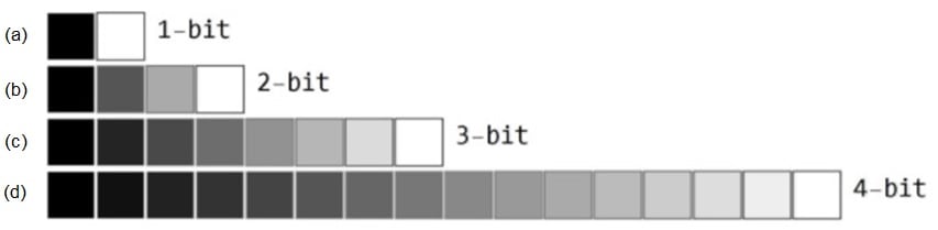
Figure 1. Available pixel intensities for 1-bit, 2-bit, 3-bit, and 4-bit image data
If n bits are used to represent a pixel, then there will be 2n pixel values ranging from 0 to (2n -1). Here 0 and (2n - 1) correspond to black and white, respectively, and all other intermediate values represent shades of gray. Such images are said to be monochromatic (Figures 1(b) through 1(d)).
A combination of multiple monochrome images results in a color image. For example, an RGB image is a combined set of three individual 2-D pixel arrays that are interpreted as red, green, and blue color components.1
Histogram
An image histogram is a graph of pixel intensity (on the x-axis) versus number of pixels (on the y-axis). The x-axis has all available gray levels, and the y-axis indicates the number of pixels that have a particular gray-level value.2 Multiple gray levels can be combined into groups in order to reduce the number of individual values on the x-axis.
Histogram of a Monochrome Image
Figure 2(a) shows a simple 4 × 4 black-and-white image whose histogram is shown in Figure 2(b). Here the first vertical line of the histogram (at gray level 0) indicates that there are 4 black pixels in the image. The second line indicates that there are 12 white pixels in the image.
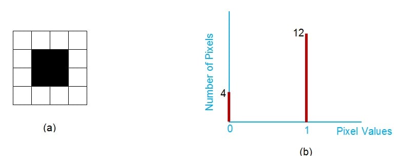
Figure 2. A black-and-white image and its histogram. Image created by Sneha H.L.
Figure 3(a) is a grayscale image. The four pixel intensities (including black and white) of this image are represented by the four vertical lines of the associated histogram (Figure 3(b)). Here the x-axis values span from 0 to 255, which means that there are 256 (=28) possible pixel intensities.
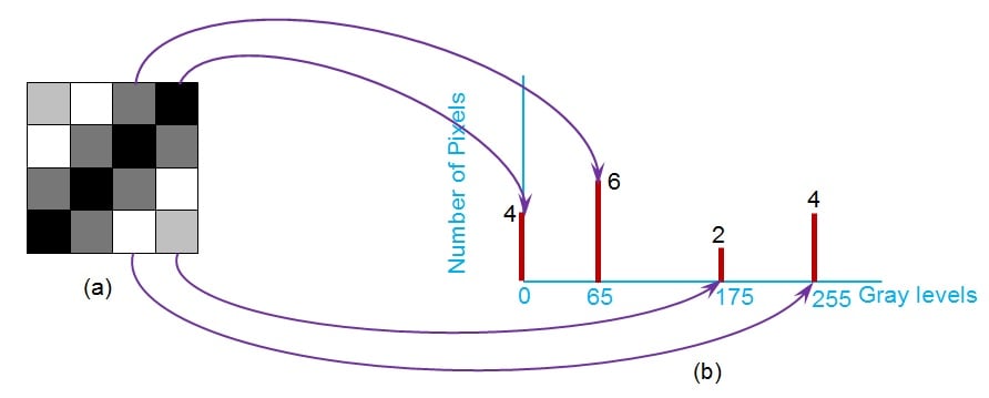
Figure 3. 8-bit grayscale image and its histogram. Image created by Sneha H.L.
Histogram of a Coloured (RGB) Image
The histogram of an RGB image can be displayed in terms of three separate histograms—one for each color component (R, G, and B) of the image. An example is shown in Figure 4. The same information can be represented also by using a 3-D histogram whose axes correspond to the red, green, and blue intensities.3
.jpg)
Figure 4. Colour image and the histograms corresponding to its red, green and blue monochrome channels. Image assembled by Sneha H.L.
Analyzing Histograms of Monochrome Images
A mere look at the histogram reveals important facts regarding its image.
1. The total number of pixels
The total number of pixels constituting the image can be obtained by adding up the number of pixels corresponding to each gray level.
2. Image brightness
You can get a general idea of the brightness of an image by looking at the histogram and observing the spatial distribution of the values. If the histogram values are concentrated toward the left, the image is darker (Figure 5). If they are concentrated toward the right, the image is lighter (Figure 6).
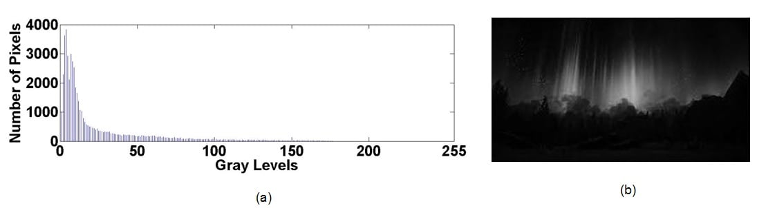
Figure 5. Histogram of a dark image. Image by Sneha H.L.
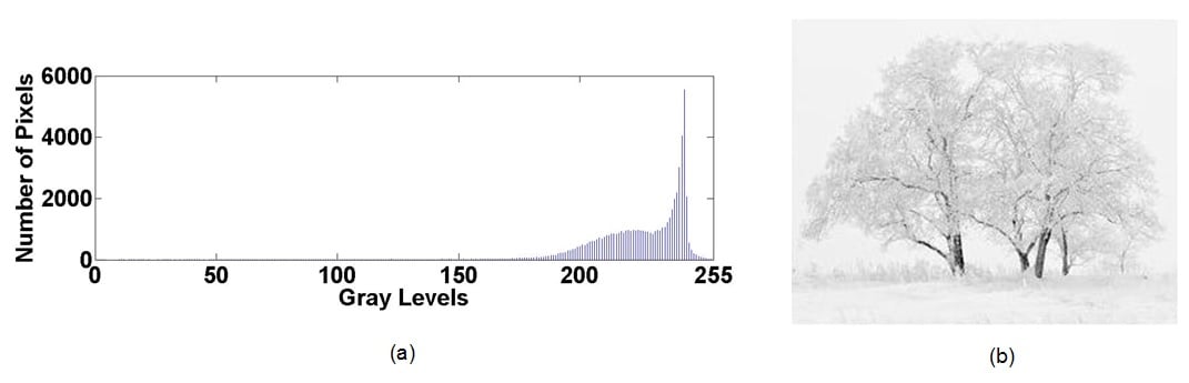
Figure 6. Histogram of a bright image. Image by Sneha H.L.
3. Contrast of the image
A histogram in which the pixel counts evenly cover a broad range of grayscale levels indicates an image with good contrast (Figure 7). Pixel counts that are restricted to a smaller range indicate low contrast (Figure 8).
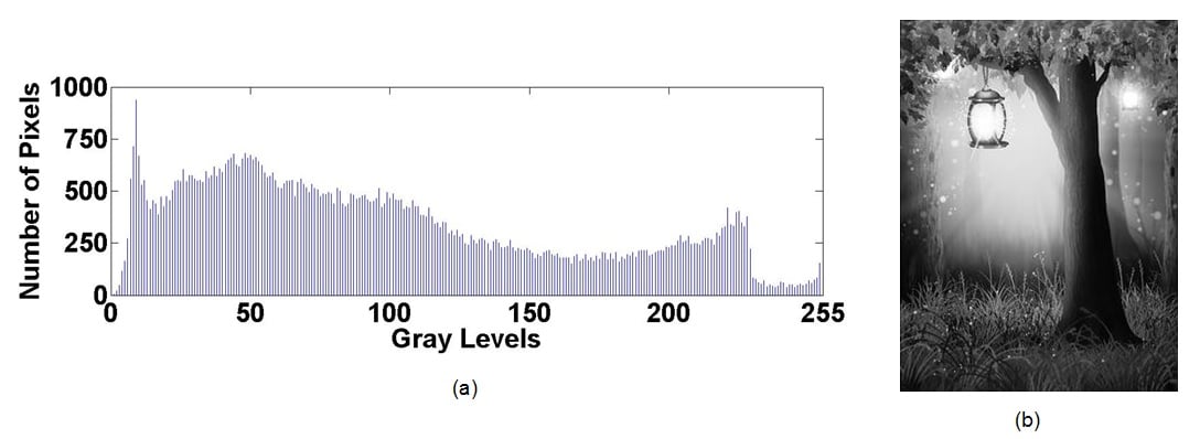
Figure 7. Histogram of a high-contrast image. Image by Sneha H.L.
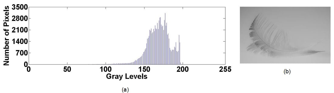
Figure 8. Histogram of a low-contrast image. Image by Sneha H.L.
4. Saturation Effects
A histogram with a prominent spike at the highest possible pixel value (Figure 9) indicates that the image’s pixel intensities have experienced saturation, perhaps because of an image processing routine that failed to keep the pixel values within their original range.
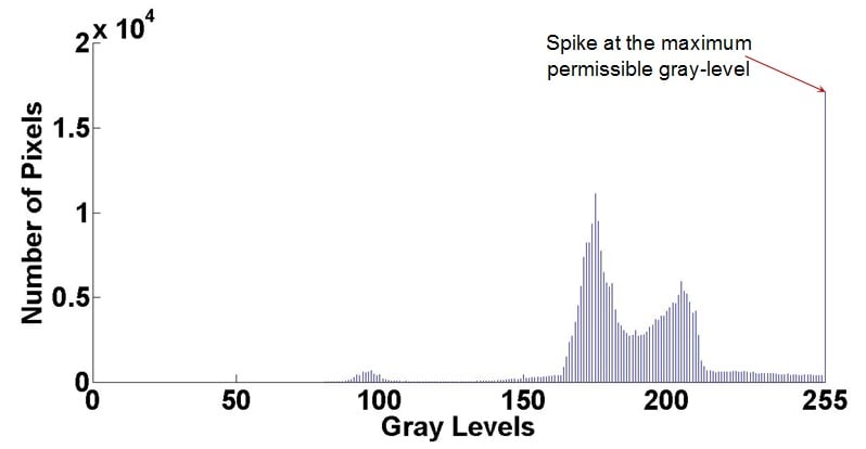
Figure 9. Histogram of a saturated image. Image by Sneha H.L.
Drawback
One limitation that we need to keep in mind is that a histogram provides no information regarding the spatial distribution of an image’s pixel values. Thus, we can have multiple different images that share the same histogram (Figure 10), and we cannot reconstruct an image from its histogram.4
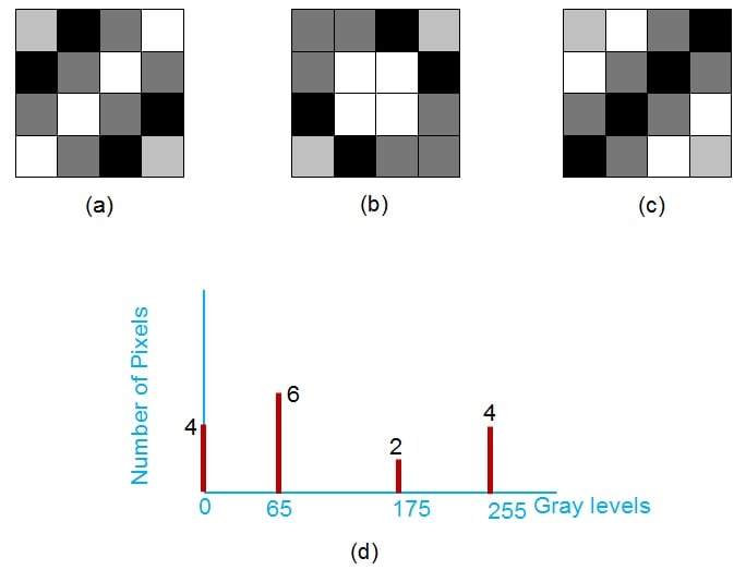
Figure 10. Different images that have the same histogram. Image by Sneha H.L.
Applications of Histogram
1. Thresholding
A grayscale image can be converted into a black-and-white image by choosing a threshold and converting all values above the threshold to the maximum intensity and all values below the threshold to the minimum intensity. A histogram is a convenient means of identifying an appropriate threshold.
In Figure 11, the pixel values are concentrated in two groups, and the threshold would be a value in the middle of these two groups. In Figure 12, the more continuous nature of the histogram indicates that the image is not a good candidate for thresholding, and that finding the ideal threshold value would be difficult.
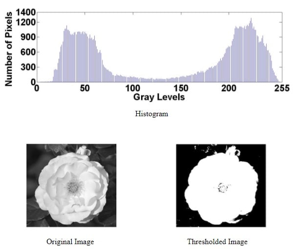
Figure 11. Histogram of the original image and thresholding results. Image by Sneha H.L.
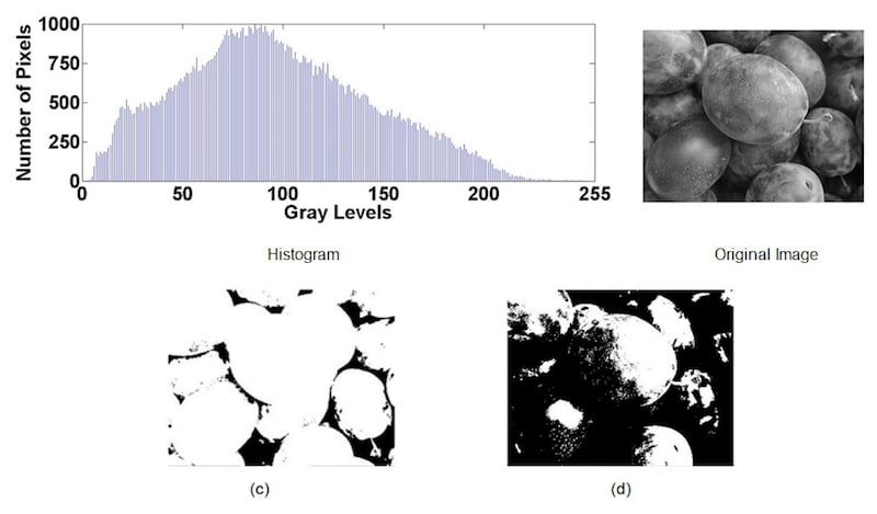
Figure 12. Histogram of the original image and two thresholding attempts. Image by Sneha H.L.
2. Image Enhancement
Image enhancement refers to the process of transforming an image so as to make it more visually appealing or to facilitate further analysis.5 It can involve simple operations (addition, multiplication, logarithms, etc.)6 or advanced techniques such as contrast stretching and histogram equalization.7
An image histogram can help us to quickly identify processing operations that are appropriate for a particular image. For example, if the pixel values are concentrated in the far-left portion of the histogram (this would correspond to a very dark image), we can improve the image by shifting the values toward the center of the available range of intensities, or by spreading the pixel values such that they more fully cover the available range.
Summary
This article has explained the essential characteristics of an image histogram, and it also discusses the histogram’s role in image processing.
References
- Digital Image Processing Using Matlab, II Edition, R.C. Gonzalez, R. E. Woods, S.L. Eddins, Gatesmark Publishing, ISBN 978-0-9820854-0-0
- https://www.tutorialspoint.com/dip/histograms_introduction.htm
- https://homepages.inf.ed.ac.uk/rbf/HIPR2/histgram.htm
- http://web.cs.wpi.edu/~emmanuel/courses/cs545/S14/slides/lecture02.pdf
- http://www.theijes.com/papers/vol6-issue6/G0606015963.pdf
- http://web.cs.wpi.edu/~emmanuel/courses/cs545/S14/slides/lecture02.pdf
- https://homepages.inf.ed.ac.uk/rbf/HIPR2/histgram.htm