Facebook
 Google
 GitHub
 Linkedin
Integrator Limitations: Magnitude and Phase Errors
In this article, we will examine the deviation of the actual transfer function H from the ideal \(H_{ideal}\) in finer detail.
In our first article on integrators, we investigated the limitations stemming from using a constant gain-bandwidth-product (constant GBP) op-amp, and we found that the best frequency range of operation is between the op-amp’s pole frequency fb and the integrator’s unity-gain frequency f0. This is the range over which the loop gain T is maximized and, hence, the range over which the deviation of the actual transfer function H from the ideal Hideal is minimized.
We now wish to examine this deviation in finer detail. Before proceeding, we recall from our second article on integrator limitations that H is affected also by the op-amp’s output impedance zo, because zo allows for signal feed-through around the op-amp.
In the following, we assume |zo| to be so much smaller than the integrator’s resistance R, that feed-through can be ignored. Under these conditions, we recycle our findings from previous articles and write, for the circuit of Figure 1(a),
\[H(j f )= \frac {V_o}{V_i} = H_{ideal}(j f) \frac{1}{1+1/T(j f)} \: \: \: \: \: \: \: \: \: \: \: \:(1)\]
where
\[H_{ideal}(j f) = \frac{-1}{jf/ f_o} \: \: \: \: \: \: \: \: \: \: \: \:(2)\]
\[f_o = \frac {1}{2 \pi RC} \: \: \: \: \: \: \: \: \: \: \: \:(3)\]
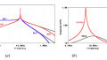
Moreover, the loop gain |T| is visualized as the difference between the open-loop gain |a| and the noise-gain |1/β| (see Figure 1(b), top), where
\[\frac {1}{\beta} = H_{ideal} +1 \: \: \: \: \: \: \: \: \: \: \: \:(4)\]
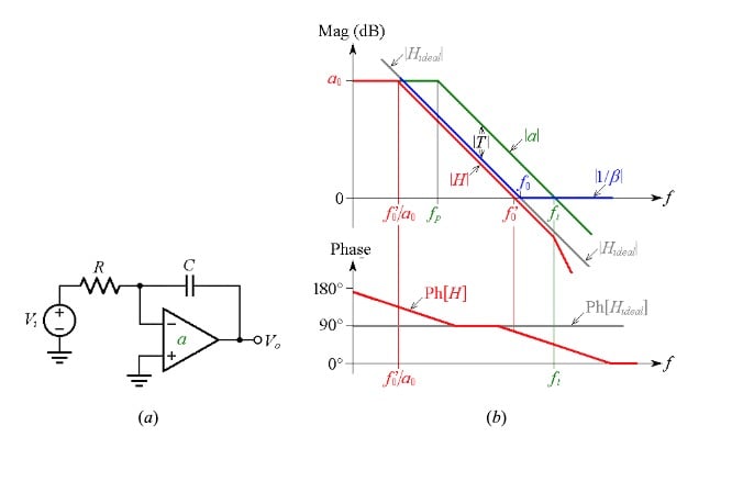
Figure 1. (a) Integrator, and (b) linearized plots of magnitude |H| (top) and phase Ph[H] (bottom).
Magnitude Error
Using Equations (1) and (2), we write
\[\left | H \right | = \left | H_{ideal} \right | \times \left | \frac {1}{1+1/T} \right | = \frac {1}{f/f_o} \times \frac {1}{\left |1+1/T \right |} = \frac {1}{f/(f_o/\left | 1+1/T \right |)}\]
indicating that magnitude-wise, the circuit still acts as an integrator, but with a unity-gain frequency of
\[f_o ' = \frac {f_o}{\left | 1+1/T \right |} \: \: \: \: \: \: \: \: \: \: (5)\]
With reference to Figure 1(b), top, we estimate |T(jf0)| by exploiting the constancy of the GBP: |T(jf0)|×f0 = 1×ft, which gives |T(jf0)| = ft/f0. Substituting into Equation (5) gives
\[f_o ' \cong \frac {f_o}{1+f_o/f_t} \: \: \: \: \: \: \: \: \: \: (6)\]
The downshift in the unity-gain frequency provides a convenient means for visualizing the departure of |H| from |Hideal|. This departure is referred to as magnitude error.
Phase Error
By Equation (2), the phase angle of the integrator is, ideally, Ph[Hideal] = Ph[–1] – Ph[j] = 180 – 90 = 90°. However, because of the integrator’s pole pair, Ph[H] will depart from 90° both at the low and at the high ends of its useful frequency range (see Fig, 1b, bottom).
We will see in the next article that the phase error in the vicinity of f0 is of particular concern in integrator-based filters such as the state-variable and the biquad filter types. This error is ϵϕ = –tan-1(f/ft). A well-designed integrator has f0 << ft, so in the vicinity of f0 we approximate as
\[\epsilon _\phi \cong -f/f_t \: \: \: \: \: \: \: \: (7)\]
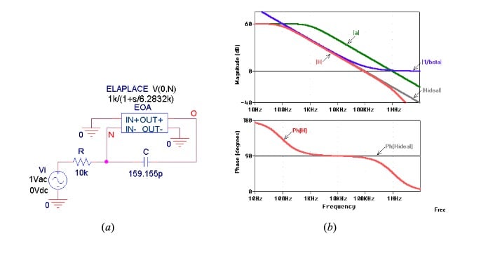
Figure 2. (a) PSpice integrator with f0 = 100 kHz and ft = 1 MHz. (b) Magnitude and phase plots.
As a practical example, consider the PSpice integrator of Figure 2(a), which uses a Laplace block to simulate an op-amp with GBP = 1 MHz. By Equation (3), f0 = 100 kHz.
Equations (6) and (7) provide the estimates \(f_o ' \cong \) 90.9 kHz and ϵϕ\((f_o ') \cong \) -5.71°, in fair agreement with the measured values of 90.53 kHz and –4.64°.
We observe that the magnitude error is not necessarily bad because we can always compensate for it by suitably predistorting the value of the RC product. For instance, lowering C from 159.155 pF to 142.473 pF in Figure 1, while leaving R unchanged, will raise f0 by the amount necessary to ensure \(f_o ' = 100.0\) kHz.
Alternatively, we can leave C unchanged and lower R from 10.0 kΩ to 8.952 kΩ.
Active Phase-Error Compensation
While the magnitude error can readily be compensated for via component-value predistortion, phase-error compensation requires that we introduce a suitable amount of phase lead to combat the phase lag due to the pole frequency ft, which is responsible for said error.
In Figure 3, this lead is provided by OA2, a matched twin of OA1. OA2 operates as a unity-gain voltage follower, so its closed-loop gain has a pole frequency of ft.
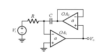
Figure 3. Active phase-error compensation circuit giving \(\epsilon _\phi \cong -(f/f_t)^3\).
A detailed analysis indicates that near \(f_o '\) we now have
\[\epsilon _\phi \cong - (f/f_t)^3 \: \: \: \: \: \: \: \: \: \: (8)\]
which, for f << ft, is clearly much better than the error of Equation (7).
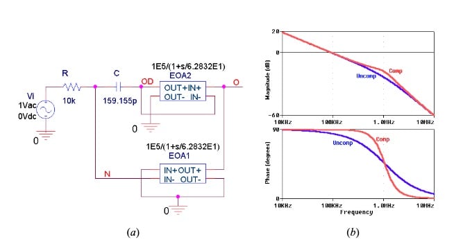
Figure 4. (a) PSpice integrator with active compensation. (b) Magnitude and phase plots.
As a practical example, consider the PSpice integrator of Figure 4(a), designed for f0 = 100 kHz and using matched op-amps with ft = 1 MHz.
Without compensation, we measure \(f_o' = 90.60\) kHz and \(\epsilon _\phi (f_o') = -4.71 \)°.
With compensation, we measure \(f_o' = 91.60\) kHz and \(\epsilon _\phi (f_o') = -0.04 \)°.
Figure 5 shows an alternative circuit for phase-error manipulation.
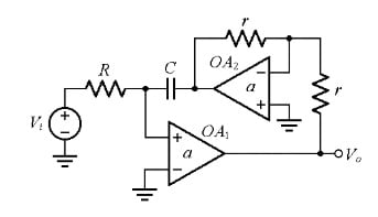
Figure 5. An alternative phase-error compensation circuit, giving \(\epsilon _\phi \cong + f/f_t\).
OA2 is now operated as a unity-gain inverting amplifier, so its closed-loop gain has a pole frequency of ft /2. Due to the inversion provided by OA2, the inputs of OA1 must be swapped, so the resulting transfer function H = Vo/Vi is that of a non-inverting integrator.
To compare its phase error to the non-compensated case, we need to plot Ph[H] + 180°, as depicted in Figure 6.
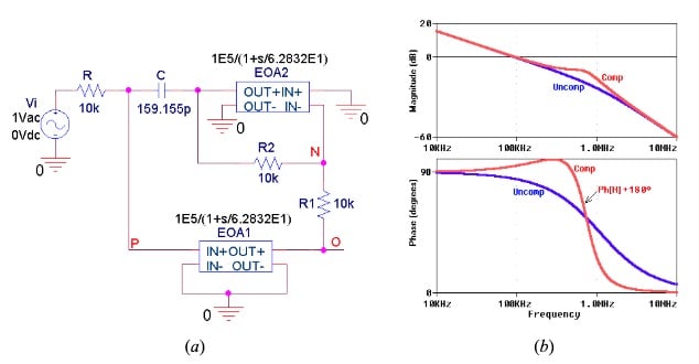
Figure 6. (a) PSpice integrator with an alternative phase compensation. (b) Magnitude and phase plots.
It can be shown that the phase error is now positive,
\[\epsilon _\phi \cong + f/f_t \: \: \: \: \: \: (9)\]
a property that comes in very handy when a compensated non-inverting integrator is connected in cascade with an uncompensated inverting type, so their opposing phase errors cancel each other out. In fact, cursor measurements in Figure 6 give \(f_o'\) = 93.48 kHz and ϵϕ (\(f_o'\)) = +4.67°, the latter being almost exactly the opposite of the uncompensated value of \(\epsilon _\phi (f_o') = -4.71\)° found in connection with Figure 4.
This concludes the third article on integrator limitations. Please share questions and comments regarding the information here in the comments below.
Related Content