 Facebook
 Google
 GitHub
 Linkedin
Unraveling the Thermocouple Approximation Error Using the Least Squares Method
Learn about the linear approximation error for a type k thermocouple and how to use the least squares method and Matlab to find the line of best fit that minimizes the approximation error.
Previously, we examined the hardware implementation of cold junction compensation (CJC) for thermocouples. CJC circuits need to sense the temperature of the cold junction (Tc) and produce a compensating voltage equal to that produced by the thermocouple at a temperature of Tc.
Overall, thermocouples are nonlinear and the compensating voltage, which is produced by a simple analog circuit, can only approximate the actual response. As a result, using a linear equation to approximate the thermocouple response introduces error to our measurements.
With all that in mind, this article will examine this error and see how we can use the least squares method to find the line of best fit that minimizes the approximation error.
Assessing the Linear Approximation Error for a Type K Thermocouple
Figure 1 below shows the output of a type K thermocouple and the linear approximation we used in the previous article.
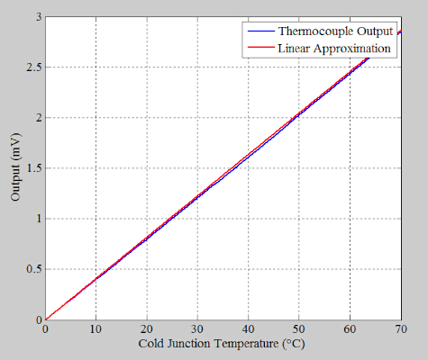
Figure 1. Output and linear approximation of a type K thermocouple.
In this case, we assumed that the slope of the thermocouple response is constant and equal to its value at room temperature (41 μV/°C at 25 °C). As shown, the employed straight line goes through the origin. By subtracting the two curves, we obtain the approximation error in μV shown in Figure 2.
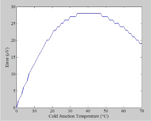
Figure 2. Graph showing the approximation error in μV.
Next, by dividing the difference curve by the slope of the straight line (41 μV/°C), we get the error in °C, which is plotted in Figure 3.
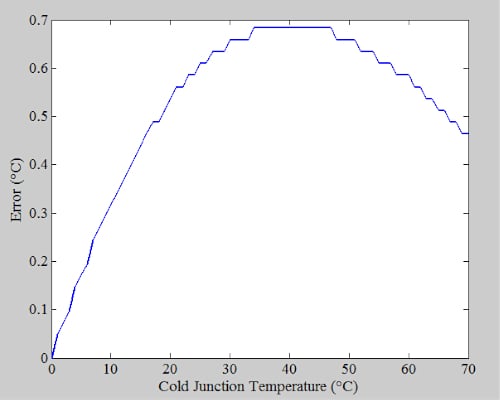
Figure 3. A graph showing the error vs. cold junction temperature.
The above graph shows that, even with ideal circuit components, we’ll have an error as large as about 0.7 °C when Tc changes from 0 to 70 °C. This error stems only from our linear approximation. We can use the least squares regression line method [video] to find a linear equation that best fits our data points.
Finding the Line of Best Fit Using Least Squares Method
We’ll explain the least squares fitting process through an example. Assume that we have the following data points:
Table 1. Example data points.
| x | 1 | 3 | 4 | 6 | 7 |
| y | 1.5 | 3 | 5.7 | 9.8 | 16 |
We want to find the straight line that best represents these data points. Figure 4 shows these points along with a straight line chosen by visual inspection that attempts to follow the trend in the data.
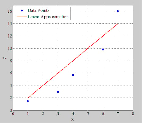
Figure 4. A plot showing the example data points and the linear approximation.
As you can see, a straight line cannot go through all these points. Therefore, our linear approximation might give values that are different from the actual values of the data points. For example, in Figure 4, the straight line gives y = 14 at x = 7, whereas the actual value is 16 at this x value. Therefore, there is a difference of 2 units between the actual value and that produced by our linear model.
In the context of the least squares method, this difference between the value of the actual curve and the linear model is called a residual (denoted by r in this article). In this example, the residual at x = 7 is equal to r = +2. The sum of the squares of the residuals can be considered as an indication of how well our linear model fits the data. With the model shown in Figure 4, we have:
\[\sum\limits^{5}_{i=1}r^{\,\,2}_{\,i}=(1.5-2)^{2}+(3-6)^{2}+(5.7-8)^{2}+(9.8-12)^{2}+(16-14)^{2}=23.38\]
Where the summation index (i) refers to the ith point in our data. The least squares method attempts to minimize the sum of the squares of the residuals for all data points by adjusting the slope (m) and y-axis intercept (b) of the linear model. The slope and y-axis intercept of the linear model that “best-fits” the data can be found using Equations 1 and 2 below:
\[m=\frac{\sum_{i=1}^{n}(x_i-\overline{x})(y_i-\overline{y})}{\sum_{i=1}^{n}(x_i-\overline{x})^2}\]
Equation 1.
and
\[b = \overline{y} -m\overline{x}\]
Equation 2.
Where:
- xi and yi are the x and y values of the ith data point
- x and y are the average values of all xi and yi
- n is the total number of data points
With the data given in Table 1, we have x = 4.2 and y = 7.2 . Table 2 shows some of the calculations when applying Equations 1 and 2 to our data points.
Table 2. Calculations for data points from Equations 1 and 2.
| i | (x, y) | \((x_{i}-\overline{x})(y_{i}-\overline{y})\) | $$(x_{i}-\overline{x})^{2}$$ |
| 1 | (1, 1.5) | 18.24 | 10.24 |
| 2 | (3, 3) | 5.04 | 1.44 |
| 3 | (4, 5.7) | 0.3 | 0.04 |
| 4 | (6, 9.8) | 4.68 | 3.24 |
| 5 | (7, 16) | 24.64 | 7.84 |
Using the above values, we obtain:
\[m=\frac{18.24+5.04+0.3+4.68+24.64}{10.24+1.44+0.04+3.24+7.84}=\frac{52.9}{22.8}=2.3202\]
and
\[b=7.2-2.3202\times4.2=-2.5448\]
From there, Figure 5 below provides a plot of the line we obtained.
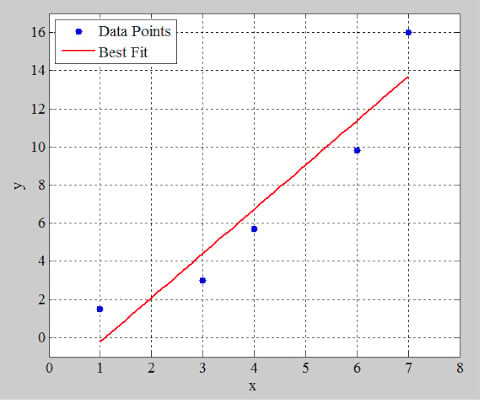
Figure 5. A plot line using Table 2's calculations.
Let’s find the sum of the squares of the residuals for this new model:
\[\sum\limits^{5}_{i=1}r^{\,\,2}_{\,i}=(1.5+0.2245)^{2}+(3-4.4159)^{2}+(5.7-6.7361)^{2}+(9.8-11.3765)^{2}+(16-13.6967)^{2}\]
This gives us:
\(\sum\limits^{5}_{i=1}r^{\,\,2}_{\,i}=13.8427\)
This equation is much smaller than the previous sum value obtained above. The calculations involved in the least squares method are tedious, and oftentimes, a spreadsheet or a computer program is used to do these calculations.
Using Matlab to Find the Line of Best Fit
After plotting a curve in Matlab, we can choose the “Basic Fitting” option from the “Tools” menu (Figure 6(a)) to open the “Basic Fitting” window (Figure 6(b)).
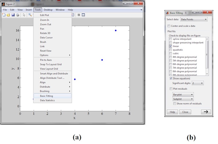
Figure 6. A Matlab screenshot showing the "best fitting" option in the Tools menu (a) and the "best fitting" window (b).
If we choose “linear” and “show equations” in the “Basic Fitting” window, Matlab will produce and display the linear equation that “best-fits” our data points.
Linear Model of a Type K Thermocouple
Continuing to use Matlab, we find the following linear model for a type K thermocouple over a temperature range of 0 to 70 °C:
Vout = 40.778 X temperature – 13.695
In this case, the slope and y-axis intercept of the model are 40.778 μV/°C and 13.695 μV. Rounding to two significant digits, we obtain:
Vout = 41 X temperature – 14
The difference between the values produced by this model and a type K thermocouple is plotted in Figure 7. This gives us the approximation error in μV.
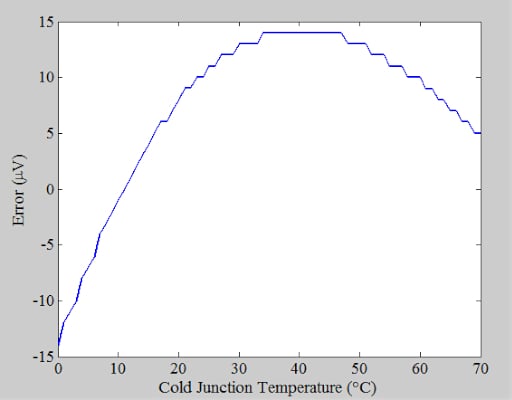
Figure 7. Plot showing the difference between values produced by the model and type K thermocouple.
Dividing these values by the slope of the line 41 μV/°C gives us the error in °C plotted below.
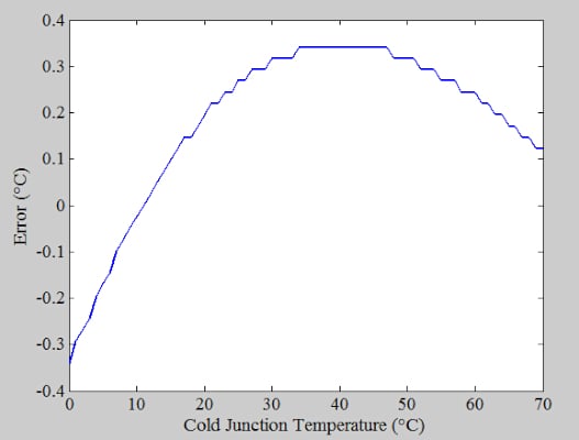
Figure 8. A plot showing the change when dividing the values of the previous plot.
With the line of best fit, the approximation error is about 0.35 °C when Tc changes from 0 to 70 °C. This is almost half the error from the previous model. As a final note, remember that you can have a more accurate model if the cold junction temperature changes in a more restricted range in your design. For example, if Tc changes from 20 to 50 °C, your line of best fit can more accurately model the thermocouple response.
For solved examples about how restricting the Tc can improve the accuracy, this application note from TI could be useful.
Featured image used courtesy of Texas Instruments
To see a complete list of my articles, please visit this page.


Thank you. But one of the signs inside brackets in the equation for the new model stays unclear to me. For example, I get “plus” in (1.5+0.2245), since (1 *2.3202 −2.5448) is negative. But why “plus” in (5.7+6.7361)?