 Facebook
 Google
 GitHub
 Linkedin
The Inverting Configuration of an Amplifier
Mentioned in the previous article, an operational amplifier is usually connected to components in a feedback circuit. In this article, we will discuss one of two amp configurations that are most widely used.
Mentioned in the previous article, an operational amplifier is usually connected to components in a feedback circuit. In this article, we will discuss one of two amp configurations that are most widely used.
Previous Article:
Characteristics of Operational Amplifiers
Inverting Configuration
As you know, operational amplifiers can be used in a vast array of circuit configurations and one of the most simple configurations to use is the inverting amplifier. The amplifier only requires the operational amplifier IC and a few other small components. Inverting amplifiers are also used as summing amplifiers, which sums the voltage present on multiple inputs and combines them into a single output voltage. Some examples are summing several signals with the same gain in an audio mixer or converting binary numbers to a voltage in a digital-to-audio-converter (DAC).
The below figure, Fig 1.1 illustrates the amplifier's inverting configuration. There are an operation amplifier and two resistors R1 and R2 inside of the inverting configuration. The second resistor, R2 is connected from terminal 3 (output terminal), back to terminal 1, which is the inverting (-) input terminal. As R2 is connected in this manner, we can apply negative feedback, which is the process of "feeding back" a small portion of the output signal back into the input terminal. However, in order to make the feedback negative, the output signal must be fed into the inverting terminal of the operation amplifier. Also, if R2 was connected between the output terminal 3 and the input terminal 2 (noninverting input), there would be positive feedback. Now the output signal is fed back into the noninverting (+) input, creating a positive feedback into the operational amplifier. If you look at the diagram closely, R2 also closed the loop surrounding the operational amp. In addition to R2 in this configuration, terminal 2 has been grounded and connected to the resistor R1 in between terminal 1 and the input signal source of voltage v1. Between terminal 3 and the ground is the point from which we will take the output since there is an impedance level that is ideally zero. Due to this, voltage v0 does not depend on the impedance value of the current that is supplied to the load impedance that is connected between the ground and terminal 3.
.jpg)
Figure 1.1 Inverted Configuration of Operational Amplifier
Closed Loop Gain in Inverting Amplifiers
Looking at Figure 1.1, we can now analyze the circuit to find what is called the closed-loop gain G, which can be written as
$$G \equiv \frac{v_{0}}{v_{1}}$$
While analyzing this circuit, the operational amplifier will be considered to be ideal for measurement purposes. Figure 1.2 (a) illustrates the equivalent closed-loop circuit, from which we can deduce that the gain A is extremely large, that of which is ideally infinite. By assuming that the circuit is producing a finite voltage at the output terminal 3, then we can say that between the operational amplifier's input terminals that the voltage is negligible and ideally zero. The output voltage v0 can be defined as
$$v_{2}-v_{1}=\frac{v_{0}}{A}=0$$
At the inverting input terminal, the voltage, v1 is given by v1 = v2. This is so because as the gain A is approaching towards infinity, v1 is approaching v2 and ideally equivalent. Having found v1, Ohm's law can now be applied to find the current i1 through R1.
$$i_{1}=\frac{v_{1}-v{1}}{R_{1}}=\frac{v_{1}-0}{R_{1}}=\frac{v_{1}}{R_{1}}$$
We need to know where this current will flow. Since the operation amplifier has an ideal infinite input impedance, which means there can be zero current drawn, it cannot flow here; instead, i1 will flow through R2 into terminal 3. From this, Ohm's law can be applied at R2 to find the value of v0.
$$v_{0}=v_{1}-i_{1}R_{2}$$
$$=0-\frac{v_{1}}{R_{1}}R_{2}$$
Then,
$$\frac{v_{0}}{v_{1}}=-\frac{R_{2}}{R_{1}}$$
.jpg)
Figure 1.2 Analysis of the inverting configuration.
This is the closed-loop gain. This gain is just the ratio of the two resistor values R2 and R1. There is a minus sign on the right side because the closed-loop inverting amplifier is providing a signal inversion. For example, if the ratio R2/R1 = 10 and a sine wave signal of 2 V is applied at the input terminal (v1), there will be a sine wave signal of 20 V (peak-to-peak) and phase-shifted exactly 180 degrees with respect to v1. Due to the fact that there is a minus sign incorporated in the ratio of the closed-loop gain, the configuration is called the inverting configuration.
A significant point worth talking about is that this closed-loop gain depends solely on external passive components (R1 and R2). This will allow the closed-loop gain to be made as accurate as needed by selected different passive components, such as resistors capacitors, or inductors, of appropriate value. Also, because of this dependency, the closed-loop gain is ideally independent of the operational amplifier gain. To summarize: the amplifier started out having a large gain A, and thus through applying a negative feedback, a closed-loop gain R2/R1 has been obtained that is much smaller than the gain but it is now stable and also predictable. I.e. gain is being traded for accuracy.
Finite Open-Loop Gain Effects
To clarify what was just said, an expression can be derived for the closed-loop gain as long as the operational amplifier's open-loop gain A is a finite value. Figure 1.3 illustrates this clarification. By denoting the output voltage as v0, the voltage between the two input terminals of the operational amplifier is now vo/A. Also, because the noninverting input terminal is grounded, this voltage at the inverting input terminal must now be -v0/A. We can write an expression for the current i1 that passes through R1 as
$$i_{1}=\frac{v_{1}-(-v_{0}/A)}{R_{1}}=\frac{v_{1}+v_{0}/A}{R_{1}}$$
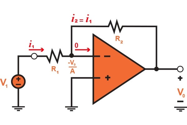
Figure 1.3 Analysis of the inverting configuration with a finite open-loop gain of the operation amplifier.
The operational amplifier's infinite input impedance drives the current i1 to flow completely through R2. Now the output voltage, v0 can be found by
$$v_{0}=-\frac{v_{0}}{A}-i_{1}R_{2}$$
$$=-\frac{v_{0}}{A}-\left ( \frac{v_{1}+v_{0}/A}{R_{1}} \right )\cdot R_{2}$$
By summing terms, the closed-loop gain G can be found by
$$G\equiv \frac{v_{0}}{v_{1}}=\frac{-R_{2}/R_{1}}{1+(1+R_{2}/R_{1})/A}$$ (1.1)
By noting that as A approaches $$\infty $$, G approaches the ideal value of -R2/R1. Looking at Fig 1.3, it can be seen that as A approaches $$\infty $$, that the voltage at the inverting input terminal will approach zero. If you recall, this was the assumption used earlier to analyze the operational amplifier when it was assumed to be ideal. Finally, we will note that Eq. 1.1 shows that in order to minimize the dependency of the closed-loop gain G on the value of the open-loop gain A, the closed-loop gain needs to be much less than the value of the open-loop gain.
Conclusion
To conclude this article, the inverting configuration has been discussed and explained. I hope that you have gained a better understanding of the purpose of this amplifier as well as how it is designed. Whether it is an audio mixer or a digital-to-audio converter, you'll find an inverting amplifier within it. Two things are to be remembered when talking about inverting amplifiers: no current flows through either input terminal and that the differential input voltage is zero (v1=v2=0). From these two rules, we derived an equation to calculate the closed-loop gain of the inverting amplifier. If you have any questions or comments, please leave them below!
Next Article in Series: Non-inverting Configuration of an Operational Amplifier
Related Content


http://www.pdfsearchengine.org
http://web.mit.edu/6.101/www/reference/op_amps_everyone.pdf
http://www.siongboon.com/projects/2008-04-27_analog_electronics/op amps for everyone third edition 2009 (Texas Instrument).pdf
weather using the inverting or level shifting (perhaps and other) configuration it has proven to be necessary to buffer the input (use the buffered input signal) to avoid “interesting” results