Facebook
 Google
 GitHub
 Linkedin
Rectifiers and Averaging Circuits
Figure 18-13 shows the standard configuration for a half-wave rectifier. It appears without much comment in dozens of textbooks. For one thing, the textbooks rarely mention that it doesn't work well with many op amps.
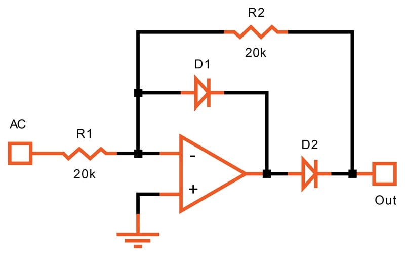
Figure 18-13. Standard op amp half-wave rectifier.
Putting a diode in the feedback path is awfully hard on the op amp. The abrupt impedance change around zero signal level can easily cause spikes and damped oscillation, affecting the accuracy.
A Bipolar Half-Wave Rectifier
Custom rectifier circuits like the one in Figure 18-14 avoid this, as well as requiring only a single supply voltage.

Figure 18-14. [click to enlarge] Bipolar half-wave rectifier.
In the circuit of Figure 18-14, the output is at ground when there isn't an input signal. It is held there by R1.
If the input moves above ground, the output follows. But if the input goes negative, there is nothing in the output stage that can pull it below ground, so it just stays there. This is illustrated in Figure 18-15. Minimum required supply voltage for a 1 V input range is 3.5 V.
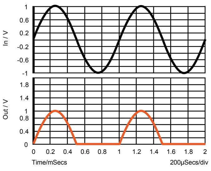
Figure 18-15. Input and output waveforms for a half-wave rectifier.
The value of R1 must be low enough to keep the voltage drop due to the base current of Q6 low. This resistor cannot be replaced with a current sink—the minimum collector-emitter voltage of an NPN transistor is too high.
You can capacitively couple the input signal. This will require connecting a resistor from the input terminal to ground to provide a DC path.
A Bipolar Full-Wave Rectifier
Next, let's consider the full-wave rectifier in Figure 18-16.
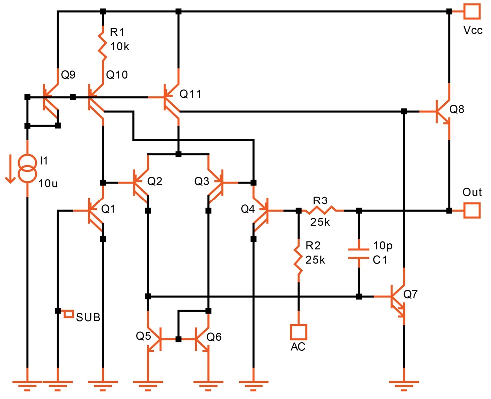
Figure 18-16. [click to enlarge] A full-wave rectifier.
In Figure 18-16, an inverting op amp configuration with a gain of 1 is used, However, it only works for negative-going input signals. As the signal moves above ground, the op amp is effectively disabled, and so the output simply follows the input. This is illustrated in Figure 18-17.
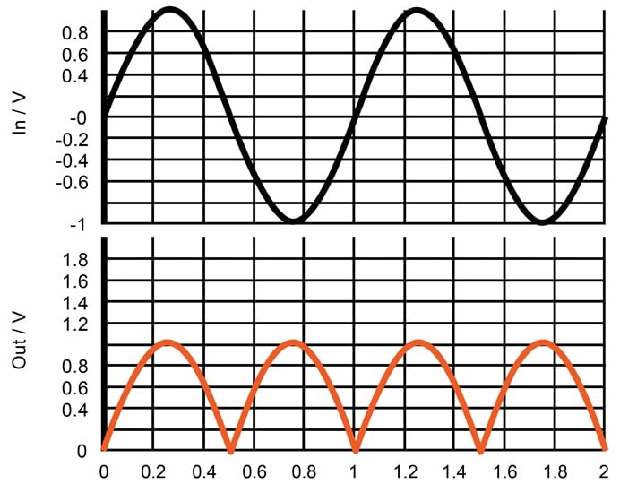
Figure 18-17. Input and output waveforms for the full-wave rectifier.
The minimum supply voltage for this circuit with a 1 Vp input is 2 V. To avoid loading down the output, a buffer needs to be used. As it happens, the same buffer circuit we employed in Figure 18-14 works here as well.
In Figure 18-16, Q10 gives a small operating current to Q1 and Q4 (about 1.7 μA). Without this, frequency compensation of the op amp becomes very difficult.
CMOS Rectifiers
Both of these circuits can be readily translated into CMOS. A CMOS version of the half-wave rectifier can be seen in Figure 18-18.
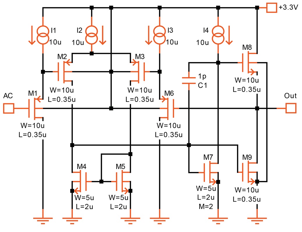
Figure 18-18. [click to enlarge] CMOS half-wave rectifier with a single supply.
This circuit takes advantage of CMOS in two ways:
- Because there's no base current, the output pull-down impedance can be quite high.
- A current sink can be used at the output instead of a resistor.
With a 1 V input range, this circuit works down to 1.8 V supply at –40 °C and 1.6 V at 0 °C. The full-wave rectifier in Figure 18-19 only needs a 1 V supply for the same input range.
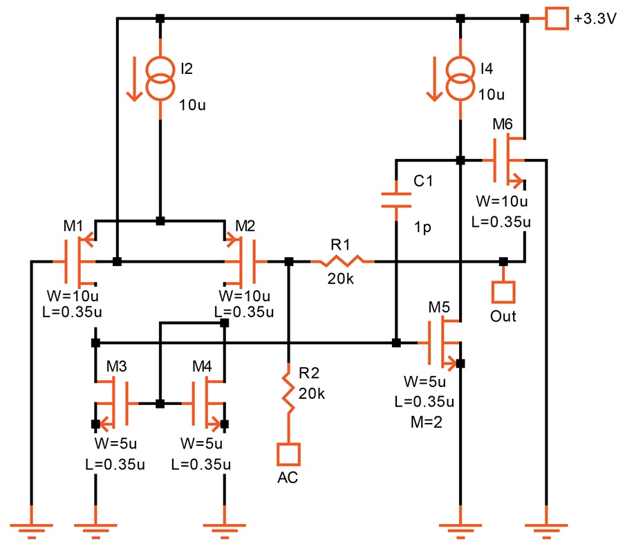
Figure 18-19. [click to enlarge] Single-supply CMOS full-wave rectifier.
Averaging Circuits
Averaging the rectified signal takes time. The longer the time constant, the smaller the ripple. However, there will always be a ripple.
Take the simplest approach, a single low-pass RC filter connected to the output. Figure 18-20 shows that a full-wave output has the advantage, producing less ripple.
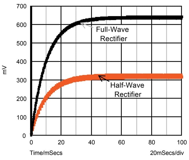
Figure 18-20. Time constant and ripple for a one-pole, low-pass filter used for averaging.
The time constant used here is 10 ms. The signal is 1 kHz. To reduce the ripple, you could increase the time constant, which means the output will take longer to reach the final level. Alternatively, you can use a higher-order filter.