Facebook
 Google
 GitHub
 Linkedin
System Notations
Video Lectures created by Tim Feiegenbaum at North Seattle Community College.
Block Diagram
First of all, what are they? They are a simplified representation of a system. They represent the relationships between functional system sections or blocks, and here is a picture of a block diagram. Let's talk about it a little more.
First of all, lines or arrows indicate flow of information or control signals. If we look at this we'll see we have lines and we have arrows, and these are indicative of the flow of information. Next item here we're mentioning is a bus. A bus is a group of wires that's served as data or address elements in a computer system. Let's take a look at here in our graph, at our picture here. We have a number of buses indicated. The blue, here, this is indicating a bus. Here, we have another bus over here. We have similar buses over here. You'll note that the buses, some of the buses, have numbers attached to them. Notice this one, 32; this one, 64; this one, 8. These are all what we would call parallel buses because they're moving. In this case there's 64 wires here. This is one example. From system memory to the microprocessor there is actually 64 physical connections, so we can move 64 bits of data at a time. We'll pick this up later in the book. Sixty-four bits is equivalent to eight bytes, so eight bytes of data can be moved to the processor at one time because there is a 64-bit data bus here.
In the same manner, here we have a 32-bit bus. This is moving data between video memory and the video display. Down here, we have an eight-bit bus that's moving data between the I/O controller and the printer. We also have some buses, notice these are indicated with just the number one. In this case, the number one wire in a bus would be indicative of a serial bus [inaudible 0:02:49] by a parallel bus.
Let's see, then we also have, here we are, control lines. These are bold single arrows pointing from the controlling block to the controlled block. We have a controlling block and a controlled block. In this particular diagram you will see... notice the large black lines here, one over here, and another one here. What these are indicating is in this case, for example, the microprocessor is controlling the video controller. The microprocessor also is controlling this thing we call the bus. The I/O controller is controlling the mouse, keyboard and printer. Here, we also have the microprocessor controller and the communication controller, in this case, it would be a modem, network interface cards, et cetera.
The block diagram, now remember, this is not a class on computers. What we're looking at here is simply a block diagram. A block diagram is useful with understanding the general nature, the general nature of a system. It provides the big picture without the detail. You notice the detail, for example, a detailed picture would've shown you those 64 lines that are just showing you that bus that contains 64 wires. A schematic diagram would've actually shown you the 64 wires. A block diagram is also helpful to gain an understanding and also to troubleshoot. Often times, if you're troubleshooting a system, a block diagram can help you to isolate the general area where a problem could be.
Flow Charts
Then we have flow charts. A flow chart is another way to describe the behavior of a system. Flow charts are useful for a number of things; for programming computers, troubleshooting complex systems, describing the operation of a system, explaining systems to users, and optimizing the design of a system. Here we have, this is in your textbook, here we have some pictures of some flow chart symbols and would give a little bit of definition of their meaning. Then, here is an actual flow chart, a simplified flow chart, for troubleshooting a computer system.
As a rule, and I note down here at the bottom, as a rule block diagrams are connected or concerned with electrical functions of the system. Block diagrams are concerned with electrical functions of a system (see: Electric vs. Electronic System). This is what we looked at on the previous slide; whereas, flow charts, which this is, are used to describe the behavior of the system. I'll just describe a couple of these. Notice here we have this rectangular box. It indicates a process used to present a process or a complete operation. Notice here, one example here is to turn on power. This would represent a complete process or operation. Then, notice here's another one. The diamond here it represents and decision. It's used to represent a branch to one of two paths based upon the indicated decision. Here's another example of this or an example of this the diamond is used, power indicator, in this case, it would probably be an LED light or something that indicates power is on. There's simply a decision is there power, is there not power. If there is power, you can continue down this stream. If there is no power, then you go over here. Is it plugged in? Is it turned on, et cetera?
The oval shape here is a terminator used as an exit point for flow chart, notice that would be down here. This would be our exit point. The off-page connector here this is used to indicate something, in this case, used to indicate a connection to a similarly labeled symbol on another page of a multipage flow chart, because often in electronic systems these flow charts become just monumental in size and you may have multiple pages to depict a flow chart.
Graphical Data
Then, graphical data. Graphical data. A graph is used to communicate technical details about the behavior of an electronic system. Many types of graphs are available. We're going to look at three of them. We're going to look at linear, logarithmic, and polar graphs. Graphs with equally spaced divisions representing the scales are called and we refer to these as line graphs or in this case a linear scale. When values on a graph fall between divisions on a scale an estimate is made of the value. This is called interpolation.
Now on the next page here we have a picture of what we call a line graph or a linear graph. The reason it is a linear graph is because both, notice here, horizontal and vertical lines have equally spaced divisions. You'll notice here the horizontal, you'll notice there is between 500 and 550 to 600, 600 to 650, 650 to 700, there is equal spacing going horizontally, and hence also going vertically there is equal spacing, and hence the term a linear graph. That word we talked about earlier on the previous slide, interpolation, is when values fall in between numbers on a given scale you must estimate. Say we wanted to know what is the value that exists at maybe this point right here and we would need to make an estimate... you would have to make the estimate based on the values that are in between, in this case, between here and between here.
Here we have a logarithmic graph. A logarithmic graph differs from a linear graph in that there is non-uniform spacing. When I say non-uniform, we have an example here, in this case, two is not midway between one and three. If you look at this graph, there are some interesting things about it. You'll note it is used to depict a very wide range of frequencies. In this case, it goes from one here all the way up to 1,000. This is in megahertz, so from one megahertz to 1,000 megahertz, so it's graphing very wide field of data. You'll notice here from one here we would step to two, and then to three. You'll notice that two usually you would expect two to be midway in between one and three, but in a logarithmic graph this simply isn't the case. You'll notice we go one, two, three, four, five, six, seven, eight, nine, and then we get to 10. Then, starting at 10, we're going to make jumps of not one but of ten. In this case it goes, 20, 30, 40, 50, 60, 70, 80, 90, and then 100. Then, from here it makes jumps of 100, 200, 300, et cetera. This is an example of what we refer to as a logarithmic graph. It is not mentioned in your text, but this graph depicts what we call a low-pass filter. It passes, in this cases, it's between about here and here, you're getting a much larger signal. This would be from about one to roughly 20 megahertz, and then from here to here is where it is what we call rolling off between about 20-40 megahertz. Then, from 100 megahertz on it is severely attenuating. It's severely diminished in size.
Then, we have the polar graph kind of like the polar bear. No, I'm kidding. All right, polar graph. This graph is of the brightness of a light emitting diode, a light emitting diode, often referred to as an LED. This is, the graph is of the brightness of the diode as it is viewed from different angles. Here you've got, this is the angular view and this is the LED. What you're graphing here is how much of the potential brightness of that LED how much of it can I see from different viewing angles. I might mention here, an LED is a device that emits light when electrical current passes through it. In this case, each of the concentric circles represents an intensity of light as viewed from zero to 90 degrees, each radial extending from this center outward corresponds to the viewing angle. As you can see here, if you're at 40 degrees, let's see what are we going to get? We're going to see about 40% of the brightness of this LED. If we were at 10 degrees off from it, we would see, in this case, 100% of its brightness. The interpretation of the data from a polar graph is the same as in the previous two graphs, the viewing angles separates the polar graph from the linear and the logarithmic.
Here, again, we have a line graph. This particular graph is very similar to the first one we looked at, is a linear graph. The difference, let's see, this graph of the FET characteristics is similar to the first graph except that it depicts a family of curves rather than just one. The first linear graph had just one single value graph. Here, we have a variety of different values graphed on this linear graph. We will talk about FETs later in this course. It is referred to as the field effect transistor.
Wiring Diagrams
Wiring diagrams. Wiring diagrams; frequently used in electronics. They are a pictorial sketch that represents the components in a circuit. Each component is labeled for clarity. The lines in the diagram represent the wires providing the electrical interconnections. We have an example here. Here is a basic wiring diagram. Again, the purpose is not to teach this system but rather just to introduce the concept of a wiring diagram. In this particular picture here we have a three-phase motor. Here we have, over here, we have the switches that will turn this motor on or off. I have a couple of different operators here that can power this motor. We're not told what this motor does but simply that is a three-phase motor. Here we have the power source and this is a three-phase AC, phases A, B and C are depicted here. This is used in usually in industrial settings. We see something here labeled K and the K's here are all tied together. These typically are indicating a relay. In this case, these relays would apply power to this particular motor. Then, we have some thermal switches here. Thermal switches act as fuses. If there is too much current being pulled by any of these phases the relay or the thermal switches would open shutting the system off. Then, we have 120 volt AC power source over here, again, another, in this case, a fuse if the system overloads. Anyway, this is a depiction of a wiring diagram.
Further Reading: Switch Types
Schematic Diagrams
Then, we have schematic diagrams. Schematic diagrams are a graphical representation based on symbols that show how all electronic components in a system are connected. Probably the key word is all electronic components. Schematic diagrams are one of the most important ways of communicating technical information about a circuit. Notice this normal behavior. Some common electrical symbols used in schematics are shown below on the following slide.
Here we see some common electronic components. We're not going to go into these at this time. Throughout this course, we will probably look at every one of these. Then, here we have a schematic of an electronic circuit. This actually comes from your simulation software that you'll be using. In this particular case, we see a number of devices depicted. Here, we have an op amp. In this case, it's a 741 op amp. We see a resistor is a one ohm resistor. Here is another resistor. Here is a capacitor. Over here we show a signal source. In this case, the signal source is a square wave at five volts coming in at 10 kHz. Here we see a ground. Down here we see a positive voltage. Here we see a negative voltage. This particular circuit is an integrator. It is a circuit that develops a ramp. It looks like this, the output of this device, but right now this is not of importance. This just is an example of an electronic circuit.
Related Content