Understanding the Noise Performance of AM Receivers with Envelope Detection

In earlier parts of this series, we studied how noise affects coherent DSB‑SC and SSB demodulators. This article continues that exploration by examining the noise performance of conventional AM, which relies on envelope detection.

 

Brief Overview of Conventional AM

In conventional AM, where the carrier is retained in the transmitted spectrum, the modulated signal may be expressed as:

$$s(t) = A_c \Big ( 1+ \mu m(t) \Big ) cos(\omega_c t)$$

Equation 1.

 

In the above equation, A_c is the carrier amplitude, m(t) is the message signal, and μ is called the modulation index. Figure 1 shows a typical output spectrum for this type of amplitude modulation.

 

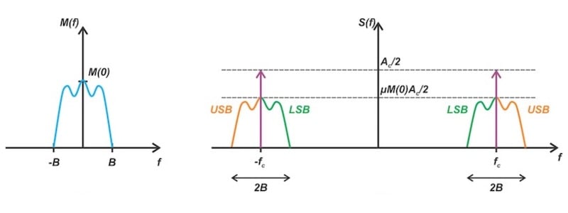
Figure 1. The spectrum of the baseband signal (a) and the conventional AM signal (b).

 

Like the DSB-SC method, the output spectrum includes two replicas of the baseband spectrum translated in frequency by ±f_c. However, unlike the DSB-SC method, the conventional AM’s spectrum includes two delta functions weighted by the factor 0.5A_c. In both DSB-SC and conventional AM, the transmission bandwidth is twice that of the message signal B_T=2B. Demodulation of conventional AM signals requires the use of an envelope detector. Figure 2 presents the basic model of an AM receiver employing this technique.

 

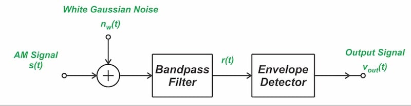
Figure 2. Block diagram of an AM receiver with envelope detection.

 

We now proceed to examine how the envelope detector affects both the input signal and the accompanying noise.

 

What Is the Power of the Modulated Carrier?

Let’s first calculate the power in the input signal s(t). Since s(t) is not periodic in practice, the average power is determined by integrating its squared value s²(t) over a very long time span:

$$P_{s,in} = \lim_{T \rightarrow \infty} \frac{1}{T} \int_{-T/2}^{T/2} s^2(t) \ dt$$

Equation 2.

 

The square of the input signal is:

$$s^2(t) = A_c^2 \Big ( 1+ \mu^2 m^2(t) + 2 \mu m(t) \Big ) \times \Big (\frac{1+ cos(2\omega_c t)}{2} \Big )$$

Equation 3.

 

The time-averages of the terms involving cos⁡(2ω_ct) are zero. Intuitively, since m(t) is a slowly varying baseband signal and cos⁡(2ω_ct) is a rapidly oscillating carrier, their product fluctuates symmetrically around zero, and thus the term m(t)·cos⁡(2ω_ct) averages out over time. A similar reasoning also applies to the product of m²(t) and cos⁡(2ω_ct). Therefore, the time average of s²(t) equals that of the following signal:

$$A_c^2 \Big ( 1+ \mu^2 m^2(t) + 2 \mu m(t) \Big ) \times \frac{1}{2}$$

Equation 4.

 

Furthermore, it’s commonly assumed that the time average of the message signal m(t) is zero. Consequently, the average power of the modulated carrier is:

$$P_{s,in} = \frac{1}{2} A_c^2 +\frac{1}{2} \mu^2 A_c^2 \times \overline{m^2(t)}$$

Equation 5.

 

The first term on the right-hand side of the above equation represents the average power of the carrier c(t)=A_c·cos(ω_ct), and the second term is the average power of the information-bearing component. The bar over m²(t) denotes its time average. For notational convenience, we denote the mean square of m(t) by P_m. This yields the following expression for the average input signal power:

$$P_{s,in} = \frac{1}{2} A_c^2 +\frac{1}{2} \mu^2 A_c^2 \times P_{m}$$

Equation 6.

 

Note that the carrier power increases the total transmitted power but doesn’t contribute to the demodulated output, as it carries no modulation information.

 

Determining the Input Noise Power

As in DSB‑SC transmission, conventional AM requires a carrier filter with a minimum bandwidth equal to twice the message bandwidth 2W. Therefore, the noise present at the carrier filter output extends over the frequency range f_c-W to f_c+W. The bandpass noise spectrum, G_n(f), is shown in Figure 3.

 

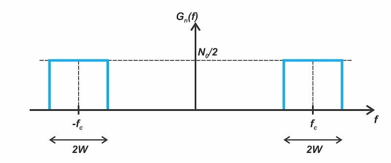
Figure 3. The noise PSD at the output of the carrier filter.

 

The average noise power equals the area under the PSD curve. Therefore, the noise power at the input of the demodulator is:

$$P_{n, in} = (\frac{N_O}{2} \times 2W) \times 2 = 2N_O W$$

Equation 7.

 

Having the input signal and noise powers, we determine the SNR at the input of the envelope detector, a parameter also known as the pre-detection SNR. By applying Equations 6 and 7, we have:

$$SNR_{in} = \frac{P_{s,in}}{P_{n,in}} = \frac{ A_c^2 + \mu^2 A_c^2 P_{m}}{4 N_O W}$$

Equation 8.

 

Signal and Noise Transformation Through the Envelope Detector

To determine the output SNR, we must understand how the signal and noise are transformed by the demodulator. Using the narrowband representation of bandpass noise, the total signal at the carrier filter output may be expressed as:

$$s(t) + n(t) = A_c \Big ( 1+ \mu m(t) \Big ) cos(\omega_c t) + n_{I}(t) \ cos(\omega_c t) - n_{Q}(t) \ sin(\omega_c t)$$

Equation 9.

 

where n_I(t) and n_Q(t) are the in-phase and quadrature components of noise, both measured with respect to the carrier wave A_c·cos(ω_ct). The phasor representation below illustrates how these signal components combine to form the noisy signal.

 

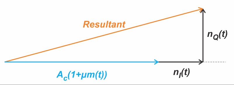
Figure 4. Phasor representation of a noisy AM signal.

 

The output of the receiver is simply the envelope of the resultant signal. Because an ideal envelope detector doesn’t respond to changes in input phase, the phase of the noisy signal can be ignored. Using the phasor diagram, the noisy signal’s envelope y(t) is obtained as:

$$y(t) = \sqrt{ \Big ( A_c + A_c \mu m(t) + n_{I}(t) \Big )^2 + \Big ( n_{Q}(t) \Big )^2 }$$

Equation 10.

 

The equation above is not immediately interpretable, since the signal and noise components are intermingled. Without simplifications, it’s impossible to separate the signal and noise contributions and obtain the additive form needed to define the signal‑to‑noise ratio.

Recall that in the case of coherent detection, as discussed in earlier articles, the demodulator output can be expressed as the sum of a signal component and an additive noise term, owing to the linear nature of the operation.

In contrast, envelope detection is inherently nonlinear, and an additive noise representation at the output is valid only when the average carrier power greatly exceeds the noise power. Assuming that the average carrier power is much greater than the noise power, Equation 10 can be approximated as follows:

$$y(t) \approx A_c + A_c \mu m(t) + n_{I}(t)$$

Equation 11.

 

Demodulation of the carrier produces a constant term A_c, which we filter out using a DC blocker. Hence, the DC blocker output is:

$$v_{out} \approx A_c \mu m(t) + n_{I}(t)$$

Equation 12.

 

With the equation in additive form, the output SNR can be readily obtained.

 

Determining Output SNR

Using Equation 12, the output signal power is given by:

$$P_{s,out} = \mu^2 A_c^2 P_{m}$$

Equation 13.

 

If the power of the bandpass noise at the input of the detector is P_n,in, then the power of each of its in-phase and quadrature components is also P_n,in. Considering this and using Equation 12, the noise power at the detector output equals that at the input:

$$P_{n,out} = P_{n, in}$$

Equation 14.

 

According to Equation 7, the noise power at the input of the demodulator is P_n,in=2N₀W. Hence, the output noise power is:

$$P_{n,out} = 2 N_O W$$

Equation 15.

 

Finally, employing Equations 13 and 15, the output SNR of the envelope detector is determined as:

$$SNR_{out} = \frac{P_{s,out}}{P_{n,out}} = \frac{\mu^2 A_c^2 P_{m}}{2 N_O W}$$

Equation 16.

 

Relationship Between Input and Output SNR

Now, by applying Equations 8 and 16 and performing straightforward simplifications, we obtain the relationship between the input and output SNR:

$$\frac{SNR_{out}}{SNR_{in}} = \frac{2 \mu^2 P_{m}}{1 + \mu^2 P_{m}}$$

Equation 17.

 

To make these ideas clearer, let’s work through an example.

 

Example: Examining the Output SNR of a Tone-Modulated AM Wave

Suppose the message signal is m(t)=cos(ω_mt) and the modulation index is μ=1. Calculate the output SNR of the AM receiver with envelope detection and compare it to that of the DSB-SC method.

 

Solution:

The average power of m(t) is 1/2 in this case. Substituting the message power and modulation index μ=1 into Equation 17 produces:

$$\frac{SNR_{out}}{SNR_{in}} = \frac{2 \times \frac{1}{2}}{1 + \frac{1}{2}} = \frac{2}{3}$$

Equation 18.

 

The DSB‑SC demodulator yields an output SNR twice the input. In this example, the envelope detector yields an output SNR equal to two‑thirds of the input SNR. Consequently, compared with a DSB‑SC coherent demodulator, the SNR is reduced by a factor of one‑third, corresponding to a performance loss of |10log⁡(1/3)|≈4.8 dB.

In other words, assuming all other factors are equal, the AM system employing envelope detection must transmit three times the power of a DSB‑SC system to achieve equivalent noise performance. Although the preceding example considered a single-tone message signal, the envelope detector’s SNR is generally lower than that achieved with DSB‑SC or SSB schemes.

 

Comparing Envelope Detector with Baseband Communication

In the previous article, we established that the SNR of both DSB‑SC and SSB methods is identical to that of the baseband system. We now compare the envelope detector to an equivalent baseband system. If the noise has a double-sided PSD of N₀/2, then the noise power at the output of the baseband receiver is N₀W. Using the received power P_s,in as established in Equation 6, the output SNR of the baseband system is expressed as:

$$SNR_{Baseband} = \frac{\frac{1}{2} A_c^2 \big (1 + \mu^2 P_{m} \big )}{N_O W}$$

Equation 19.

 

Now, dividing the envelope detector’s output SNR (Equation 16) by the baseband SNR, we obtain:

$$SNR_{out} = \frac{\mu^2 P_{m}}{1 + \mu^2 P_{m}} \times SNR_{Baseband}$$

Equation 20.

 

This result demonstrates that the envelope detector’s SNR is consistently lower than that of the baseband system. This is because a significant portion of the transmitted power is devoted to the carrier component, which conveys no modulation information.

If the modulation index μ in Equation 20 is allowed to grow indefinitely, the fraction approaches unity and the output SNR converges to that of the baseband system. From the conventional AM signal expression (Equation 1), a large μ implies that the carrier power becomes negligible compared with the sideband power, in which case the system effectively reduces to a DSB‑SC scheme.

In practice, the modulation index typically lies in the range of 0.8–0.9. The average message power depends on the source; for speech signals with a wide dynamic range, it is about 0.1. Using these representative values, the fraction in Equation 20 evaluates to approximately 0.07, which corresponds to a performance loss of ∣10log⁡(0.07)∣≈11.5 dB.

 

Threshold Effect

The analysis above was carried out under the assumption that the average noise power is small compared to the carrier power at the envelope detector input. When this assumption doesn’t hold, the analysis becomes substantially more complex. While the detailed analysis is outside the scope of this article, we’ll nevertheless outline a few of its results. Figure 5 illustrates the phasor representation of a noisy AM signal with high noise relative to the carrier.

 

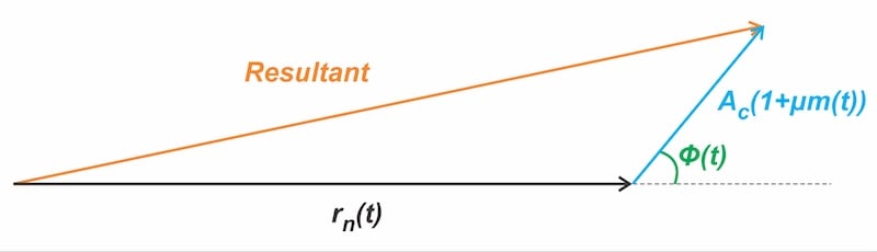
Figure 5. Phasor representation of a noisy AM signal when the noise is strong relative to the carrier.

 

In the diagram above, r_n(t) represents the envelope of the noise and ϕ(t) is its phase. As observed, the noise vector, which is the dominant component, is chosen as the reference. Therefore, the signal component A_c·(1+μm(t)) is rotated by ϕ(t) to account for the phase difference between noise and signal. Assuming the noise is significantly stronger than the carrier, the phasor representation can be used to approximate the envelope of the noisy signal as follows:

$$y(t) \approx r(t) + A_c \big [1 + \mu m(t) \big ] cos[\phi(t)]$$

Equation 21.

 

As seen, the output doesn’t contain the message scaled by a constant but instead multiplied by cos[ϕ(t)]. Because the phase of the narrowband noise, ϕ(t), is uniformly distributed over 2π radians, the message information is lost at the envelope detector's output. Mathematical analysis reveals that as the carrier‑to‑noise ratio (CNR) falls below about 10 dB, the envelope detector’s SNR decreases at a rate exceeding that of the high‑CNR regime.

This behavior is termed the threshold effect. For this reason, conventional AM systems are typically operated above the CNR threshold to prevent significant degradation in SNR. For a more detailed discussion of the threshold effect in conventional AM, see Section 2.12 of Communication Systems (4th edition) by Simon Haykin.

 

Wrapping Up

In this article, we analyzed the noise performance of conventional AM systems using envelope detection. Our analysis showed that because envelope detection is nonlinear, the additive noise model holds only when the carrier power greatly exceeds the noise power, and even then, the output SNR remains lower than that of DSB-SC or SSB, since a substantial share of the transmitted power is spent on the carrier rather than the message. Together with the earlier articles in this series, this completes our comparison of noise performance across coherent and noncoherent AM demodulation schemes.