Project

Gathering and Analyzing a Robot’s Accelerometer Data

September 01, 2017 by Robert Keim

An accelerometer can be a valuable addition to a robotics project. This article will show you one approach to generating and analyzing acceleration data.

Supporting Information

The Accelerometer

In a previous article I introduced the Romi robot chassis from Pololu and a custom-designed Romi-control PCB. You can use the following link to download the full schematic and the BOM.

RomiRobotControlBoard_schematic_and_BOM.zip

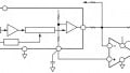
This PCB includes, among other things, an accelerometer. The part I chose is the ADXL326 from Analog Devices. It’s a three-axis, analog-output device and, from the perspective of the user, it’s not at all complicated. As you can see, few external components are required:

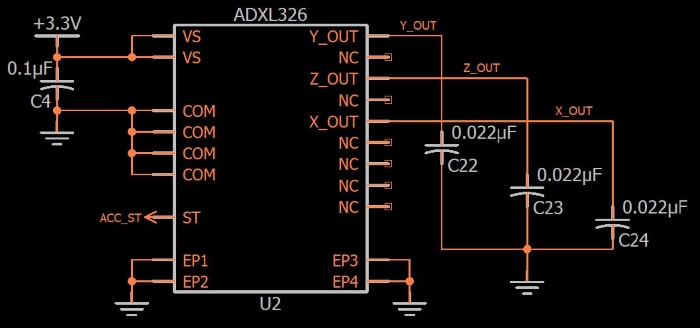
The only real design effort involved is choosing the value of the three output capacitors (C22, C23, and C24). Each of these caps forms a low-pass filter with an internal ~32 kΩ resistor; thus, by choosing an appropriate capacitance value you can limit the bandwidth of the analog outputs according to the needs of your application.

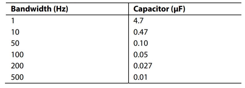
Table taken from the ADXL326 datasheet.

My caps are (nominally) 0.022 µF, so based on the table above my bandwidth will be slightly higher than 200 Hz.

The following diagram conveys the ADXL326’s x, y, and z directions.

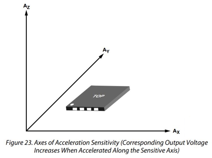
Diagram taken from the ADXL326 datasheet.

The Romi control PCB has the accelerometer oriented as follows:

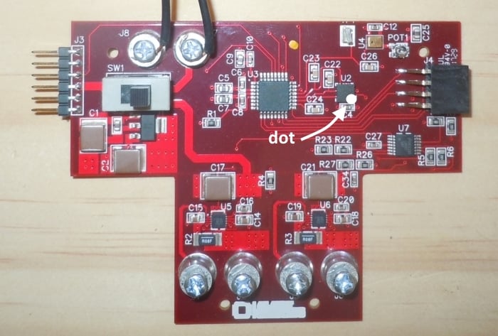
If we combine this orientation with the datasheet diagram and the robot movement directions as defined here, we can determine that

the robot’s forward direction corresponds to negative x-axis acceleration,
the reverse direction corresponds to positive x-axis acceleration,
the rightward direction corresponds to positive y-axis acceleration,
and the leftward direction corresponds to negative y-axis acceleration.

The ADC

We will use the EFM8’s analog-to-digital converter to digitize the three analog acceleration signals generated by the ADXL326. We’ll use the full 14-bit resolution and the internally generated 2.4 V reference. You can refer to the hardware configuration file and the ADC.c source file for ADC configuration details; these, along with all other source and project files, can be downloaded by clicking the following link:

AccelerationData_Source_and_Project_Files.zip

If you look at the full schematic you’ll notice that the accelerometer output signals are connected directly to the ADC inputs. No anti-aliasing filter is needed because bandwidth limitation is accomplished by the low-pass filter discussed above, and I’m pretty sure that we don’t need a voltage follower because the ADC module has a selectable-attenuation module that presumably includes some sort of circuitry that results in low output impedance.

We’ll use the ADC’s autoscan functionality to collect 2400 bytes of ADC data. Each sample requires two bytes and we have three channels (for three axes), and thus we have (2400/2)/3 = 400 samples per axis.

Transferring Data

We need to get the acceleration data to a PC for visualization and analysis. In the past I have used a USB-capable microcontroller in conjunction with a custom Scilab script (see this article, including the links in the “Supporting Information” section). However, I’ve decided to move to a simpler and more versatile system. The previous approach certainly has advantages, but it’s restrictive (because you have to use a microcontroller with USB functionality) and complicated (because of the additional USB firmware and all the Scilab development).

The new method relies on YAT (“Yet Another Terminal” program) and Excel. I assume that other spreadsheet software could be used, but the instructions here are specific to Excel.

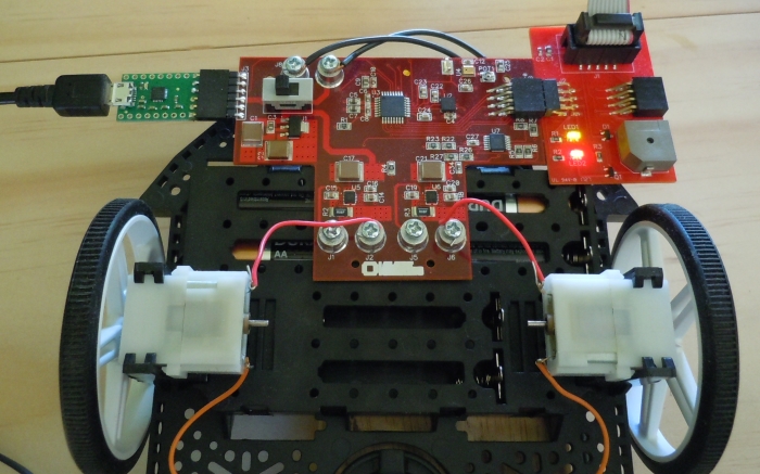
I appreciate the simplicity of UART communication but computers don’t have serial ports anymore. The simplest remedy to this situation is a USB-to-UART converter; I’m using this one from Pololu. It’s essentially a breakout board for the CP2104 from Silicon Labs; I could design my own but if Pololu sells theirs for $5.95, why bother. This handy little board allows me to write firmware as though USB doesn’t exist—just send a byte, receive a byte, like in the good old days of RS-232.The following photo shows the Romi control PCB connected to the C2 adapter board on the right and the USB-to-UART converter on the left.

Note: If you’re powering the board from USB, you should ensure that your code doesn’t allow the motors to be enabled. USB ports aren’t designed for that sort of current draw. I recommend physically disconnecting the motors, just to be sure.

When the ADC has finished the 1200 samples (400 per axis), we simply write each byte out the serial port, as follows:


void Transfer_ADCBuffer(unsigned int num_bytes)
{
	unsigned int n;

	SFRPAGE = UART0_PAGE;

	SCON0_TI = 0;	//make sure that the transmit interrupt flag is cleared

	for(n=0; n

The ADC is configured to sequentially sample from P1.5, then P1.6, then P1.7, back to P1.5, and so forth.

<img alt="" src="https://www.allaboutcircuits.com/uploads/articles/proj_AccData_ADCchannels.JPG" />

As you can see from the schematic, this results in data that is arranged in memory as follows: z-axis, y-axis, x-axis, z-axis, y-axis, x-axis, and so forth. The ADC is configured for big endian, which means that each sample will begin with the high byte. Thus, our memory looks like this:

<img alt="" src="https://www.allaboutcircuits.com/uploads/articles/proj_AccData_memory.JPG" style="border:1px solid rgb(205, 205, 205)" />

`YAT`

If everything is working correctly, the ADC data will appear in the YAT window. Here is what you need to do to make it very easy to inspect this data and work with it in Excel:

Go to Terminal->Settings and select “Binary” for “Terminal Type.”
In the same window, click “Binary Settings”; check the box for “Separate settings for Tx and Rx” then enter “6” for “Break lines after” in the “Rx” section.

<img alt="" src="https://www.allaboutcircuits.com/uploads/articles/proj_AccData_binarysettings.JPG" style="border:1px solid rgb(205, 205, 205)" />

Back in the main window, click on the “10” button so that the data appears as decimal

<img alt="" src="https://www.allaboutcircuits.com/uploads/articles/proj_AccData_decimal.JPG" style="border:1px solid rgb(205, 205, 205)" />

Now when you transfer the data, it will appear as follows:

<img alt="" src="https://www.allaboutcircuits.com/uploads/articles/proj_AccData_YATmonitor.JPG" style="border:1px solid rgb(205, 205, 205)" />

This is the format we want: each row consists of one data point, i.e., one two-byte sample for each acceleration axis.

`Excel`

First, save the YAT data to a file:

<img alt="" src="https://www.allaboutcircuits.com/uploads/articles/proj_AccData_savetofile.JPG" style="border:1px solid rgb(205, 205, 205)" />

Now you can import this space-separated data into Excel using the “From Text” button in the “Data” ribbon. Note that this block of data will remain “connected” to the data file, so to bring in new data you simply use the “refresh” functionality (see the video below for a demonstration).

Once you have the raw data in Excel, you can convert it to ADC counts and to volts (or millivolts). I have my worksheet set up like this:

<a href="https://www.allaboutcircuits.com/uploads/articles/proj_AccData_Excelsheet.JPG" target="_blank"><img alt="" src="https://www.allaboutcircuits.com/uploads/articles/proj_AccData_Excelsheet.JPG" style="border:1px solid rgb(205, 205, 205)" /></a>

`<em><a href="https://www.allaboutcircuits.com/uploads/articles/proj_AccData_Excelsheet.JPG" target="_blank">Click to enlarge</a></em>`

On a separate sheet, I have a plot that pulls data from the “millivolts” columns. If you want to use my Excel file, feel free:

<a class="downloadable" href="https://www.allaboutcircuits.com/uploads/articles/Three-Axis_Accelerometer_Data.zip">Three-Axis_Accelerometer_Data.zip</a>

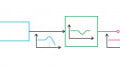
Here is a plot of “self-test” output signals (you can read about the self-test functionality in the ADXL326 <a href="http://www.analog.com/media/en/technical-documentation/data-sheets/ADXL326.pdf" target="_blank">datasheet</a>).

<img alt="" src="https://www.allaboutcircuits.com/uploads/articles/proj_AccData_selftest.JPG" />

(The initial rising edge is a result of the accelerometer’s startup delay.) Self-test causes the analog outputs to assume a predetermined value; if the measured voltages correspond to the expected voltages, you know that the accelerometer is functional. And because the predetermined value is different for each axis, self-test allows you to confirm that you are associating the samples with the correct axis.

Here are plots for two more data sets. In the first, the PCB is not moving; in the second, I am using my hand to jiggle the robot chassis.

<img alt="" src="https://www.allaboutcircuits.com/uploads/articles/proj_AccData_noacceleration.JPG" />

<img alt="" src="https://www.allaboutcircuits.com/uploads/articles/proj_AccData_jiggle.JPG" />

The following video helps to clarify the overall procedure:

<iframe allowfullscreen="" frameborder="0" height="315" src="https://www.youtube.com/embed/-cqmqTXNvLw?rel=0&showinfo=0" width="560"></iframe>

`Summary`

We discussed the hardware implementation of a three-axis, analog-output accelerometer, and I presented a straightforward method of getting stored accelerometer data from the robot’s microcontroller to a PC. We then moved the data into Excel and plotted the results.