 Facebook
 Google
 GitHub
 Linkedin
How to Check and Calibrate a Humidity Sensor
How accurate is your humidity sensor? Find out with this project.
How accurate is your humidity sensor? Find out with this project.
Humidity sensors are commonplace, relatively inexpensive, and come in many different varieties. Too often, we check the datasheet, use them with an interface, and (as long as the values “look reasonable”) we accept the results.
In this project, we demonstrate how to go a step further and verify the accuracy of a humidity sensor. We also illustrate a general method for sensor calibration and apply the method to calibrate the results to improve the accuracy of the humidity measurements.
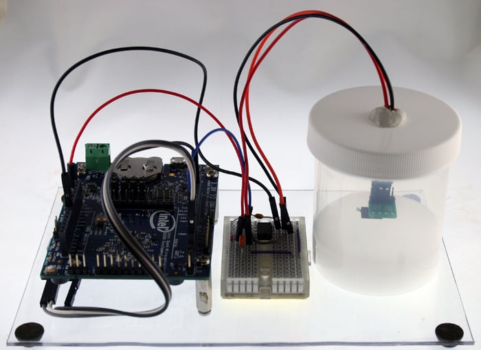
Testing setup used in the project (left to right, Quark D2000 microcontroller board, sensor interface, HIH5030 sensor in a micro-environment).
Project Fundamentals
To check the accuracy of a sensor, obtained values are compared to a reference standard. To check the accuracy of a humidity sensor, we use the “saturated salt” method to produce the standards. Put simply, certain salts (i.e., ionic compounds such as table salt or potassium chloride), when dissolved in an aqueous solution, produce an atmosphere of a known humidity (see reference PDF).
These chemical properties are used to create micro-environments of known relative humidity (RH) percentages (i.e., reference standards), and the sensors are read inside the micro-environment. Specifically, we will make a solution in a sealed jar to preserve the atmosphere and then place the connected sensor in the sealed jar. Subsequently, the sensor is repeatedly read and the values recorded.
By repeating the procedure using several different salts, each producing a different relative humidity, we can develop a profile for the sensor under test. Since we know what the relative humidity is for each micro-environment, we can assess the deviations of our sensor readings from those known values, and thus, evaluate the accuracy of the sensor.
If the deviations are substantial, but not insurmountable, we can apply mathematical calibration procedures in software to increase the accuracy of the measurements.
A Word about Safety
Before going further, it is essential that you handle the chemicals used in this project responsibly.
- Read the safety data sheet (SDS, or sometimes MSDS (material safety data sheet)) for each of the chemicals used (links for the SDS for each salt used are provided below, and you can also conduct literature searches on each salt and their safe handling procedures).
- Do not inhale or ingest the chemicals.
- Do not let the chemicals contact your skin or eyes (use gloves and goggles).
- Do not prepare the solutions in the same area that food is prepared.
- Properly store the chemicals.
- Properly discard the solutions and all of the instruments used to prepare the solutions so that exposures do not take place accidentally.
- Before starting, know what to do if an accidental exposure takes place (see the safety datasheet).
Salts Used
In general, the more RH atmospheres that you can produce for reference standards, the better the characterization of the sensor under test will be. There is, however, always a limit on resources in a practical sense. In this project, four reference standards were used and the salts used to produce the reference standards were chosen to cover a range of possible RH values, but also with consideration to safety, availability, and cost.
The salts below were chosen. In the case of sodium chloride (table salt), pure kosher salt was obtained cheaply at a local grocery store. If you go that route, avoid using table salt with additives, such as iodine or anti-caking agents.
| Salt | % RH (at 25°C) | Source | Safety Data Sheet |
|---|---|---|---|
| Lithium Chloride | 11.30 | Home Science Tools | SDS for LiCl |
| Magnesium Chloride | 32.78 | Home Science Tools | SDS for MgCl |
| Sodium Chloride | 75.29 | Various (see text) | SDS for NaCl |
| Potassium Chloride | 84.34 | Home Science Tools | SDS for KCl |
Creating a Micro-Environment
We have standards for nearly everything and there is even one for creating a stable RH from an aqueous solution (see ASTM E104 - 02(2012)). While my bench, and probably yours, is not an official testing laboratory, it is worthwhile to follow the specifications in the standard as closely as you can.
Note also that the results presented in this project, while collected with care, should not be construed as reflecting or indicating an overall quality statement of the accuracy of any brand of sensor. Only a small number of sensors were tested and those used had different ages and different usage histories.
For each salt, a slushy mixture was created by adding distilled water to a consistency similar to very wet sand. Four or five tablespoons of chemical and one tablespoon of distilled water can be tried, but you may have to do a little experimenting.
The mixture was made in a small jar with a tight seal. Glass or even plastic should work well, so long as it can keep the atmosphere inside. A small hole can be made in the top of the jar to run connecting wires to the sensor interface and then to a microcontroller. The connected sensor is then positioned approximately 0.5-1.0 inch above the mixture. Take care that the sensor never directly contacts the solution or it will likely be damaged. To hold the connection in place and to seal the hole in the cap, some easily removable contact putty can be used.
It is important that you allow plenty of time for equilibration before you take the final reading. I tested this issue empirically, taking readings every minute for up to six hours in selected test cases. In my experience, this was longer than needed and I settled on 90-120 minutes equilibration time for each sensor and salt. Then an average of the last five readings were used for the final value. For all cases, the five values showed very little, if any, difference.
Additionally, all readings were taken at about 25° C (± 1°) ambient temperature, and the RH value used for each standard was that listed for 25° C (see this PDF for the values).
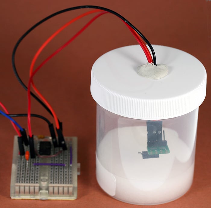
HIH5030 sensor on a carrier board inside a micro-environment containing sodium chloride.
Hardware
Microcontroller
In this project, we interface the sensors using a Quark D2000 microcontroller. The D2000 is a 3V board with I2C and analog-to-digital interfaces. For more information on the D2000, the reader is directed to these previous AAC articles:
- Introducing the Intel D2000 Quark Microcontroller Developer Kit
- The Quark D2000 Development Board: Moving Beyond “Hello World”
- Quark D2000 I2C Interfacing: Add a Light Sensor and an LCD
- Quark D2000 I2C Interfacing: Add a Color Sensor and Asynchronous Mode
Keep in mind, though, that most any other microcontroller with the appropriate interfaces can be used.
Sensor Interfaces
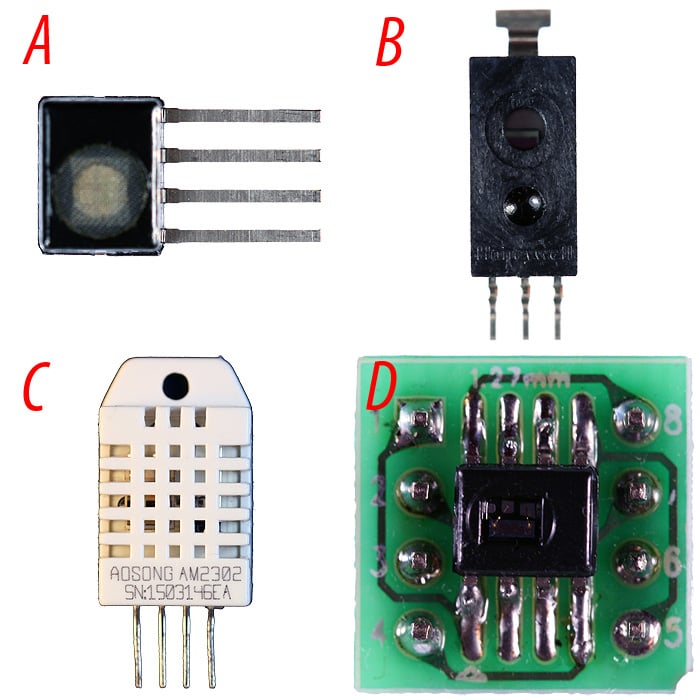
Sensors tested in the project; A) HIH8121, B) HIH5030, C) DHT-22 (AM2302), D) HIH6030 (on a carrier board).
Four different types of humidity sensors were tested: DHT-22 (two were used), HIH5030, HIH6030, and HIH8121.The schematics below illustrate the simple interfaces used for each type of sensor, and consultation with the linked data sheets will provide background information for the circuits.
- The DHT-22 is a temperature and humidity sensor with a proprietary serial output (see this AAC article for more information on the serial protocol used).
- The HIH5030 is a humidity sensor with analog (voltage) output. The interface for this sensor uses an op-amp in a unity-gain configuration for impedance matching.
- The HIH6030 and HIH8121 are temperature and humidity sensors that use the I2C protocol (see this AAC article for more information on the I2C communication procedures used).
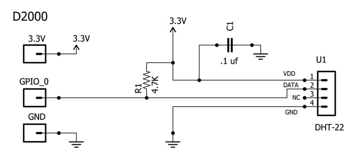
DHT-22 to D2000 interface.
DHT-22 BOM: U1, DHT-22 sensor; R1, 4.7kΩ resistor; C1, 0.1 µF capacitor.
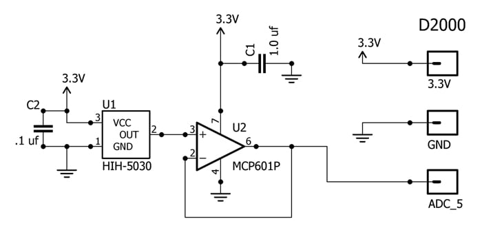
HIH5030 to D2000 interface.
HIH5030 BOM: U1, HIH3050 sensor; U2, MCP601P op-amp; C1, 1.0 µF capacitor; C2, 0.1 µF capacitor.
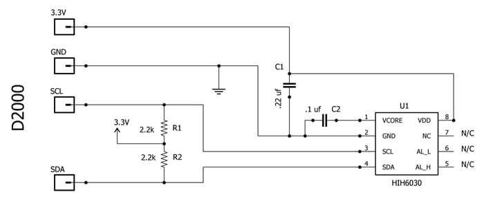
HIH6030 to D2000 interface.
HIH6030 BOM: U1, HIH6030 sensor; R1 and R2, 2.2 kΩ resistor; C1, 0.22 µF capacitor; C2, 0.1 µF capacitor.
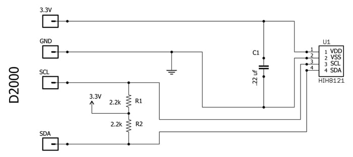
HIH8121 to D2000 interface.
HIH8121 BOM: U1, HIH8121 sensor; R1 and R2, 2.2 kΩ resistor; C1, 0.22 µF capacitor.
Sensor Software
All of the programs for gathering sensor data are written in the C language and can be downloaded by clicking on the “Humidity Sensor Project Code” button. Each is commented and straightforward. For each sensor, the program simply reads the sensor every minute and sends the value to a serial monitor. As such, they should be easy to adapt to your particular application.
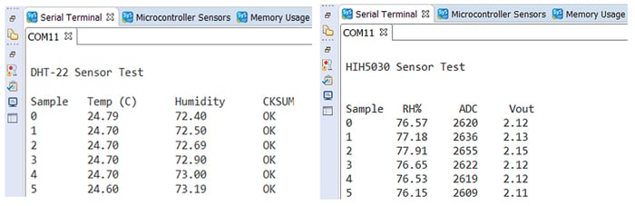
Screenshots of output from DHT22.c (left) and HIH5030.c (right).
Program files for the project can be downloaded by clicking the link below.
Sensor Evaluation Procedure
The table below contains the data from evaluating the sensors in each of the four micro-environments.
| DHT #1 | DHT #2 | HIH5030 | HIH6030 | HIH8121 | ||||||
|---|---|---|---|---|---|---|---|---|---|---|
| Reference RH | OBS | ERR | OBS | ERR | OBS | ERR | OBS | ERR | OBS | ERR |
| 11.30 (LiCl) | 12.56 | 1.26 | 16.29 | 4.99 | 13.02 | 1.72 | 20.79 | 9.49 | 12.31 | 1.01 |
| 32.78 (MgCl) | 32.36 | -0.42 | 33.79 | 1.01 | 33.46 | 0.68 | 40.77 | 7.99 | 32.43 | -0.35 |
| 75.29 (NaCl) | 73.04 | -2.25 | 74.50 | -0.79 | 77.74 | 2.45 | 83.83 | 8.54 | 76.63 | 1.34 |
| 84.34 (KCl) | 82.30 | -2.04 | 82.15 | -2.19 | 85.84 | 1.50 | 93.43 | 9.09 | 85.01 | 0.67 |
| RMSE | 1.657 | 2.799 | 1.708 | 8.796 | 0.920 | |||||
Once you have collected the data from the sensor performance in stable environments of known relative humidity, you can numerically evaluate a sensor’s accuracy.
Note that in the table, we calculated the error for each sensor at each RH standard. We can’t, however, simply average those values to evaluate the sensor because some values are positive and other values are negative. If we simply took an average, the resulting value would minimize the average error since the positive and negative values would cancel each other.
Instead, we calculate a root mean square error (RMSE) to characterize the sensor’s accuracy. The formula for RMSE is below:
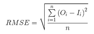
where O is the observed sensor value and I is the ideal sensor value (i.e., the reference standard). To calculate RMSE, we square each error (the deviation from the reference standard), then calculate the arithmetic average of those values, and finally, take the square root of the average.
Once you have characterized the accuracy of the sensor, you can use the RMSE to decide whether it is necessary to calibrate the sensor. In some cases, the RMSE is small and completely acceptable for your application and you can reasonably decide that no calibration is required.
For example, the results for the HIH8121 are impressive. The RMSE is less than 1% and all sample points have an error less than 2%.
On the other hand, in some cases, you may find that the sensor response is so poor and irregular that you simply decide that another sensor is required for your application.
The decision to calibrate should always take into consideration the degree of accuracy necessary for the task. Nevertheless, we can improve the accuracy of the sensor readings by calibration, for all of the sensors in the table.
Sensor Calibration Procedure
To calibrate a sensor, we need to first mathematically determine the function that relates the ideal values to the observed values. A linear regression procedure can be used to determine that function.
The word “linear” in the name of the regression procedure does not mean a linear function. Instead, the term refers to a linear combination of variables. The resulting function can be linear or curvilinear. All three of the polynomial functions below represent linear regression (note: we are ignoring a 0 degree case which is not useful in this context).
- y = ax + b (first degree, linear)
- y = ax2 + bx + c (second degree, quadratic)
- y = ax3 + bx2 + cx + d (third degree, cubic)
In the current project, we calculate sensor values using four reference standards (i.e., n = 4). Thus, a third-degree polynomial is the highest-degree polynomial that we can calculate. It is always the case that the highest-degree polynomial possible is n - 1, and in this case that means 3 (4 - 1).
Least-squares procedures are ordinarily used for linear regression. In this procedure, a line is fit such that the sum of the distances from each datum to the line is as small as possible. There are many programs available that use least squares procedures to perform linear regression. You can even use Excel (click here for more information).
It should also be noted that we do not have to use linear regression. We could use nonlinear regression. Examples of nonlinear regression result in a power function or a Fourier function. Linear regression, however, is well-suited to our project's data and, further, software correction (calibration) is easily implemented. In fact, in this project, I don’t believe you would gain much of anything by using nonlinear regression.
Choosing the Polynomial
In theory, we want to use the polynomial that best fits the data. That is, the polynomial that produces the smallest coefficient of determination, denoted r2 (or R2, pronounced “R squared”). The closer r2 is to 1, the better the fit. With least squares estimation, it is always the case that the higher the degree of polynomial used, the better the fit.
You do not, however, have to automatically use the highest-degree polynomial possible. Since calibration will take place in software, there may be cases in which the use of a lower-degree polynomial represents a speed and/or memory advantage, especially if the accuracy to be gained by using a higher-degree polynomial is very small.
Below, we demonstrate the calibration procedures for the HIH6030 sensor using polynomials of different degree, and in so doing we will illustrate the general procedure which is applicable to any degree of polynomial that you choose to use.
Using the data from the previous table, we first perform the least squares regression procedure to determine the coefficients for each polynomial. Those values will come from the regression software package used. The results are below, including the r2 values.
- Linear: y = ax + b; a = 1.0022287, b = -8.9105659, r2 = 0.9996498
- Quadratic: y = ax2 + bx + c; a = -0.0012638, b = 1.1484601, c = -12.0009745, r2 = 0.9999944
- Cubic: y = ax3 + bx2 + cx + d; a = 0.0000076, b = -2.4906103, c = 1.2061971, d = -12.7681425, r2 = 0.9999999
The observed values can now be modified using the calculated functions. That is, the sensor readings can be calibrated as illustrated in the table below (note that OBS, Corrected, and ERR values are rounded to two decimal places).
| RAW | 1st Degree | 2nd Degree | 3rd Degree | |||||
|---|---|---|---|---|---|---|---|---|
| Ref RH | OBS | ERR | Corrected | ERR | Corrected | ERR | Corrected | ERR |
| 11.30 | 20.79 | 9.49 | 11.93 | 0.63 | 11.36 | 0.06 | 11.30 | 0.00 |
| 32.78 | 40.77 | 7.99 | 31.95 | -0.83 | 32.83 | 0.05 | 32.78 | 0.00 |
| 75.29 | 83.83 | 8.54 | 75.11 | -0.18 | 75.85 | 0.55 | 75.29 | 0.00 |
| 84.34 | 93.43 | 9.09 | 84.73 | 0.39 | 84.83 | 0.49 | 84.34 | 0.00 |
| RMSE | 8.795736 | 0.562146 | 0.371478 | 0.00212 |
It can be seen that all three of the polynomials produced a significant decrease in the RMSE, compared to the observed measures, and that is why you calibrate. The graph below illustrates the improvement using the 1st degree polynomial. Note how the calibrated (corrected) data points now lie near the ideal diagonal.
.jpg)
Scatter plot of output from an HIH6030 sensor.
Calibration in Software
Once we have run the calibrations and chosen the polynomial, we can modify the software to incorporate the corrections into the sensor data. Using the HIH6030.c example, we can modify the program code as follows:
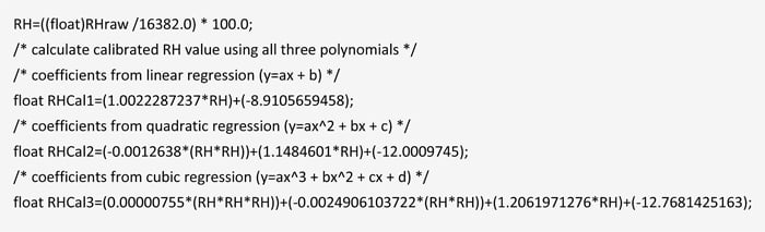
The initially calculated variable is RH. In the code lines above, we have created three new variables representing calibration (RHCal1, RHCal2, RHCal3). For illustration, we have created new variables using each of the three polynomials, whereas, in practice, you would likely calibrate the sensor value using only the chosen polynomial.
Summary Example
To summarize the steps for checking and calibrating a humidity sensor, a final example is presented using data from the DHT-22 (#2) sensor that was evaluated.
- The first step is to evaluate the sensor performance using reference standards.
This was done using the salts in micro-environments to produce atmospheres with known RH. The data were collected and appear in a table previously presented. We can characterize sensor accuracy using the RMSE term, which also appears in the table. Based on the results of the first step, we can decide whether to perform sensor calibration. If so, then proceed to the second and third steps.
- The second step is to perform linear regression to determine a function that relates the ideal RH value (from the standards) to the observed value from the sensor readings.
Here, we chose a cubic polynomial (y = ax3 + bx2 + cx + d, where y is the calibrated value and x is the sensor reading) and determined that the coefficients are a = 0.000091367, b = -0.01452993, c = 1.77623089, and d = -14.17403758.
- The final step is to modify the sensor values using the polynomial to calculate the calibrated values.
The modifications (calibrations) are implemented in software and translate the sensor readings to their calibrated equivalents.
The graph below illustrates the result of the steps. The plot includes the observed values as well as the calibrated values (for the data collected) that are derived from the calibration polynomial.
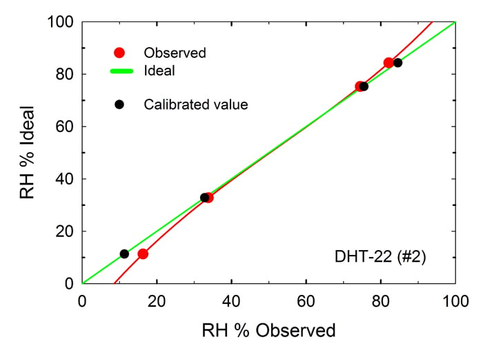
Scatter plot of output from a DHT-22 sensor.
Closing Thoughts
In this project we demonstrated a method for evaluating the accuracy of common humidity sensors. That is, by utilizing chemical properties to develop reference standards, we can compare the sensor readings to standard values and independently determine the accuracy of the sensors. Furthermore, we demonstrated a software procedure for calibrating the sensor readings and thereby producing more accurate measures of relative humidity.
Sensor evaluation and calibration are procedures relevant anywhere that sensors are used. In the case of humidity sensors, this project demonstrates relatively inexpensive and easy methods of adding to their value.


Excellent article. Kudos!
I never knew about the salts trick. I made a calibration chamber using the wet bulb/ dry bulb technique. This is an excellent article.
Thanks so much for the kind words.