 Facebook
 Google
 GitHub
 Linkedin
Analyzing 2nd-Order Circuits in Laplace Space Using Python
Learn about simplifying the mathematics of circuit analysis using the Laplace transform, Python, and SymPy using a series RLC circuit as an example.
Studying electrical circuits can be a very slippery slope. Before you know it, you’re knee-deep in differential equations. This can be scary to folks who feel uncomfortable with calculus. However, I often tell my EE students that being an engineer isn’t about getting good at solving hard problems the hard way; instead, it’s mostly about finding easier ways to solve them. This kind of logic is useful when I teach classes on circuit analysis and need to motivate them to learn the Laplace transform.
Transforming time-dependent differential equations to Laplace space ensures that the solution of those differential equations is reduced to an algebraic exercise; no calculus is needed! However, sometimes the amount of algebra involved in determining the solution can negate the method's benefits, making students wish they were doing more advanced math. One solution, however, is Python. Utilizing Python can dramatically reduce the amount of algebra needed to determine the solution.
In this article, we'll first walk through an example, show how the Laplace space comes into play, and how Python can help get through the math easier.
Example: Finding Current in a Series RLC Circuit
Before jumping into how Laplace space and Python come into play within circuit analysis, let's set up the example to the point where the Laplace transform enters.
First, consider how the current flowing through a capacitor is proportional to the derivative of the voltage across that capacitor concerning time. Similarly, the voltage across an inductor is proportional to the derivative of the current flowing through that inductor concerning time:
$$ v_L = L\frac{di_L}{dt}$$
Equation 1a.
$$i_C = C \frac{dv_C}{dt}$$
Equation 1b.
These differential relationships are fundamental to describing and analyzing the current and voltage behavior in a circuit such as the one shown in Figure 1.
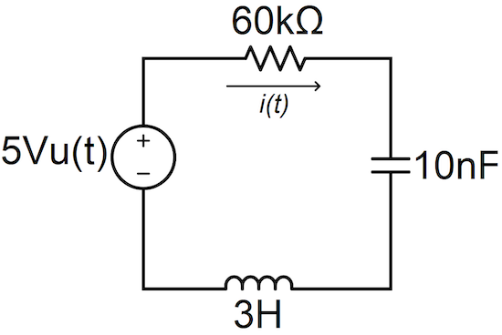
Figure 1. An example RLC circuit.
In the RLC circuit of Figure 1, we see that the currents flowing through the elements are all equal because the elements are all in series. Also, at t ≥ 0, the voltage across this circuit's passive elements is equal to 5 V (the DC source voltage). We can write these relationships as Equations 2 and 3.
$$ i_L = i_C = i_R $$
Equation 2.
$$v_R + v_L + v_C = V_{dc}$$
Equation 3.
Combining Equations 1a and 1b with Equations 2 and 3 yields Equation 4, which is an integro-differential equation describing the temporal behavior of the current flowing through the circuit shown in Figure 1.
$$u(t)5V=(3H)\frac{di}{dt}+(60k\Omega)i+\bigg(\frac{1}{10nF}\bigg)\int{idt}$$
Equation 4.
Taking the derivative of both sides of Equation 4 concerning time and rearranging the coefficients for the differential terms yields Equation 5, the differential equation describing the transient behavior of the current in the circuit of Figure 1.
$$\frac{5V\delta(t)}{3H}=\frac{d^2i}{dt^2}+\bigg(\frac{60k\Omega}{3H}\bigg)\frac{di}{dt}+\bigg(\frac{1}{3H\cdot10nF}\bigg)i$$
Equation 5.
Let’s pause and reflect on what we’ve just done. So far, we haven’t really had to do much calculus. Basically, we’ve described the current evolution in this circuit over time, but we haven’t solved the functional form of that current for time. If we were to proceed in the time domain, we would need to determine whether this circuit is overdamped, underdamped, or critically damped. Then, having chosen a general form for our solution, we would need to apply boundary conditions to that general solution and its derivative for time to determine the values of several constants in the general form of the solution.
That’s the simplest, most straightforward way to solve for current in a 2nd-order circuit if we stay in the time domain. However, we can avoid the messiness of the time domain (i.e., most of the actual calculus) if we transform Equation 6 into Laplace space.
$$\mathcal{L}\{f(t)\} =F(s)=\int_{0^-}^\infty f(t)e^{-st}dt$$
Equation 6.
Now that we've reached this point in our example, let's get a brief overview of the Laplace space.
The Laplace Space—Laplace Transform Properties and Pairs
At this point, depending on your educational background (or your faded memory of college courses), you might be wondering, “what is Laplace space?” I’ll leave a more complete description to mathematicians, but for our purposes, you can think of Laplace space as a complex frequency domain. Functions in Laplace space contain rich information about changes over time, which can be manipulated with simple algebra to extract that temporal information.
The single-sided Laplace transform is generally performed via integration according to Equation 6. This equation defines the Laplace-transform of f(t), F(s), as the result of integrating the product of f(t) and e-st from t = 0- to infinity. In addition, inverse-transforming from s-space to the time domain is performed according to Equation 7.
$$\mathcal{L}^{-1}\{F(s)\} =f(t)=\frac{1}{2\pi j}\int_{\epsilon-j\infty}^{\epsilon+j\infty} F(s)e^{st}ds$$
Equation 7.
You can always perform those integrals to transform from s-space to t-space and back again, but integration is a pain, and the inverse Laplace transform integral requires us to ensure the value of $$\epsilon$$ lies within the region of convergence for that integral; we should really dust off our complex analysis skills to execute that integral properly. Fortunately, Laplace transforms and inverse transforms can usually be performed using tables of the linear properties of Laplace space and by referencing a table of transform pairs without needing to integrate at all.
Figures 2a and 2b show minimal versions of these, though more complete Laplace tables can be found with an internet search.
![]()
Figure 2a. Laplace transform properties.
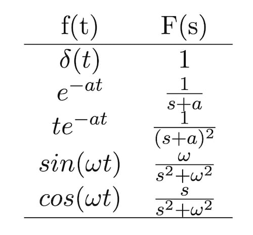
Figure 2b. Laplace transform pairs.
Now that we've had that refresher, let's dive back into our example.
Solving for Current in Laplace Space
Applying the Laplace transform properties to each term of our time-dependent Equation 6 yields the s-space Equation 8. It's important to note that I’m assuming here that the current just before t = 0 was 0A and that it had been that way for a while.
$$s^2I(s)+\bigg(\frac{60k\Omega}{3H}\bigg)sI(s)+\bigg(\frac{1}{3H\cdot10nF}\bigg)I(s)=\frac{5V}{3H}$$
Equation 8.
With that in mind, we can easily manipulate Equation 9 algebraically to find I(s). Then, determining i(t) is as simple as inverse-transforming I(s). This simplicity is the reason why we perform circuit analysis in Laplace space; it’s an amazingly quick way to solve hard problems.
$$I(s) = \bigg(\frac{5V}{3H}\bigg)\bigg(\frac{1}{s^2+\big(\frac{60k\Omega}{3H}\big)s+\big(\frac{1}{3H\cdot10nF}\big)}\bigg)$$
Equation 9.
From here, things can get a bit messy. It’s true that we can perform the inverse transform by reversing the process we used to transform from the time domain to s-space using the tables of Figure 2. However, we need to algebraically manipulate the expression for I(s) until it conforms to one or a sum of many of the functions in our transform pair table in Figure 2b. If done by hand, that process can involve so much tedious algebra that it entirely negates the benefits of solving circuits in Laplace space instead of solving differential equations in the time domain.
Using Python and SymPy to Perform the Inverse Laplace Transform
At this point in our example, we’ve done all the real circuit work by hand. It’s time to pull out the computing power of Python and SymPy to do the inverse transform for us.
First, we need to open a Python environment. I use Google Colaboratory to solve these problems because it’s web-based, all the libraries I need are available, and it renders any visual output alongside the commands. This program is similar to a Jupyter notebook, but it’s maintained by Google.
Step 1, we’ll import the SymPy library and define our symbols—s and t:
from sympy import *
s,t = symbols(‘s,t’)
Considering Equation 9, we can define I(s) in terms of our symbol ‘s’:
i = 5/(3*(s**2 + 20000*s + 33333333))
Finally, we perform the inverse transform of I(s) into the time domain and print the result onto the notebook using the following command:
inverse_laplace_transform(i, s, t).simplify()
Which then produces Equation 10:
$$\frac{5\sqrt{66666667}(e^{2\sqrt{66666667}t}-1)e^{-t(\sqrt{66666667}+10000)}\theta(t)}{400000002}$$
Equation 10.
Note that the Heaviside step function is represented in this expression as θ(t). Equation 10 is not the form we want, exactly, because SymPy tries to maintain fractional representations rather than rounding irrational numbers. However, with a little manipulation on paper, we can rewrite i(t) as Equation 11:
$$i(t) = 0.1mA (e^{-1835t}-e^{-18165t})u(t)$$
Equation 11.
Where u(t) represents the step function.
With all of that done, we're finished. Using that example, that’s how you can solve for an unknown, time-dependent quantity in a 2nd-order circuit using Laplace space, with the help of Python and the SymPy library.
How Else Can Python Help With Circuit Analysis?
While the scope of this article is limited to the use of Python to perform the inverse Laplace transform in analyzing 2nd-order circuits, the SymPy library in Python can be used to help solve many types of circuit analysis problems. Anytime algebra is involved, you can employ Python to mitigate the tedium. The best approach, I believe, is to apply all the necessary circuit principles (Kirchhoff’s laws, Ohm’s law, etc.) by hand. Then, use Python to finish the process when you’ve reduced your problem to an equation or system of equations on paper. Circuit analysis in Laplace space is an arena in which the strengths of this approach are on full display. By using a computer to perform the inverse transform, we can dramatically reduce the amount of manual algebraic manipulation necessary to obtain a solution, and the beauty and benefits of Laplace space are preserved.
Related Content


Is it just me, or does equation 7 seem wrong? The last part is duplicated from the previous equation.