Explore the Y Factor Method for Noise Figure Measurement

The NF metric allows us to characterize the noise performance of RF components and systems. The ability to make accurate NF measurements can carry a significant dollar value for chip manufacturers because accurate measurements are required to guarantee that a premium product actually meets the specified noise performance and, thus, can be sold at a premium price. Therefore, we shouldn’t be surprised to find that a significant amount of research has been carried out over decades to improve the methods of noise figure measurement. One popular technique is the Y factor method, which is the focus of this article.

 

Noise Figure Measurement Using a Two-port Device

Consider a two-port device connected to a source resistance, R, at a temperature of T, as shown below in Figure 1.

 

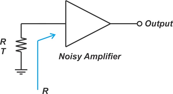
Figure 1. A diagram of a two-port device connected to a source resistance.

 

The total output noise, N_o, against the source resistance temperature, T, is plotted in Figure 2.

 

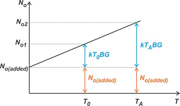
Figure 2. Plot showing the total output noise vs. the source resistance temperature.

 

If R_S were noiseless—i.e., T = 0 K—the only noise that appeared at the output would have been that of the device under test denoted by N_o(added). As we increase the temperature of R_S, its noise contribution rises. Finding the noise figure of the device is actually equivalent to finding the above “noise line”. There are two ways to specify a line: through two points that lie on the line; or through a single point and the line’s slope. The Y factor method actually measures two points from the noise line and uses that information to find the noise factor of the device under test (DUT). An alternative noise figure measurement method is the cold-source method that determines the noise factor by finding a single point on the line as well as the slope of the line (kBG).

With that in mind, let's take a look at the Y factor method.

 

Using the Y Factor Method to Find the Noise Factor

Figure 3 shows the basic block diagram for the Y factor method. 

 

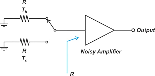
Figure 3. Block diagram of the Y factor method.

 

To find two different points of the noise line, we need to apply two different noise levels to the input. The required input noise powers are produced by connecting two matched resistors at temperatures T_c and T_h to the DUT’s input. For the Y factor method, it is easier to model the DUT’s noise performance through its equivalent noise temperature, T_e. If the output noise added by the DUT is N_o(added), its noise temperature is given by:

 

\[T_e=\frac{N_{o(added)}}{kBG}\]

 

Where k is Boltzmann’s constant, and B and G are the bandwidth and available power gain of the DUT. Modeling the component’s noise through its noise temperature, we can easily find the output noise for the two input noise levels. The output noise power for the hot source at T_h is given in Equation 1.

 

\[N_{h}=kT_hBG+kT_eBG\]

Equation 1.

 

Similarly, the output noise for the cold source, T_c, is found via Equation 2.

 

\[N_{c}=kT_cBG+kT_eBG\]

Equation 2.

 

In the above set of equations: 

• T_e and the product BG are unknown
• The noise temperature of the two inputs, T_h and T_c, is known for having a high degree of accuracy 
• N_h and N_c are measured values

If we divide Equation 1 by Equation 2, the term BG drops out, and we get Equation 3.

 

\[Y= \frac{N_{h}}{N_{c}}=\frac{T_h+T_e}{T_c+T_e}\]

Equation 3.

 

This ratio is known as the Y factor. Using a little algebra, the above equation gives us the noise temperature of the DUT in Equation 4.

 

\[T_e = \frac{T_h - YT_c}{Y-1}\]

Equation 4.

 

Having T_e, we can apply the following equation to find the noise factor:

 

\[F= 1 + \frac{T_e}{T_0}\]

 

The Calibration Step—Calibrating Noise and Receiver Noise Temperature

The Y factor method is straightforward in principle. In practice, however, there are some intricacies that require careful attention. One of these intricacies is the noise added by the measuring equipment. This is illustrated in Figure 4 below.

 

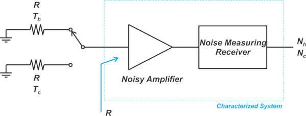
Figure 4. Block diagram showing a noisy amplifier and a noise-measuring receiver.

 

As the above figure highlights, the measured output noise powers, N_h and N_c, are affected by the noise from the measuring equipment. In other words, by substituting N_h and N_c into Equations 3 and 4, we’re actually finding the noise temperature of the two-stage cascaded system made of the DUT and the measuring equipment. Applying Friis’s equation, the noise temperature of a two-stage cascaded system gives us Equation 5.

 

\[T_{cas} = T_{DUT} + \frac{T_{Receiver}}{G_{DUT}}\]

Equation 5.

  

Where: 

• T_DUT and T_Receiver are the noise temperature of the DUT and the measuring equipment
• G_DUT is the available power gain of the DUT

When the DUT gain exceeds 30 dB, we can neglect the noise from the second stage and assume that T_cas ≃ T_DUT. However, when this condition is not satisfied, we have to use a calibration step to correct the error produced by the second stage. During the calibration step, the noise source is directly connected to the “noise measuring receiver,” and the Y factor method is applied to determine the noise temperature of the receiver (Figure 5). 

 

Figure 5. Block diagram showing the Y factor method applies to find the receiver's noise temperature.

 

Applying the hot and cold noise power to the measuring equipment, we obtain two points from the noise line of the calibration system, N_{h, cal} and N_{c, cal}. Now we can find the Y factor for the calibration setup:

 

\[Y_{cal}= \frac{N_{h, \text{ } cal}}{N_{c, \text{ }cal}}=\frac{T_h+T_{Receiver}}{T_c+T_{Receiver}}\]

 

By rearranging the above equation, we obtain the receiver noise temperature:

 

\[T_{Receiver} = \frac{T_h - Y_{cal} T_c}{Y_{cal}-1}\]

 

To summarize, the calibration step (Figure 5) measures the instrument itself and determines T_Receiver. Next, with the DUT in place (Figure 4), the noise temperature of the cascaded system T_cas is found. Finally, assuming that the DUT’s gain is known, we substitute T_Receiver and T_cas into Equation 5 to obtain T_DUT. Most often, the DUT’s gain is unknown. However, the above measurements can be used to readily find G_DUT. 

 

Calculating the Device Under Test Gain

The noise powers obtained from the measurement setup—N_h and N_c in Figure 4—experience the DUT’s gain; however, N_{h, cal,} and N_{c, cal} don’t experience this gain (Figure 5). Therefore, G_DUT can be estimated by Equation 6.

 

\[G_{DUT} = \frac{N_h - N_c}{N_{h, \text{ } cal}-N_{c, \text{ }cal}}\]

Equation 6.

 

In a previous article, we discussed that the power gain used in the noise figure definition is the available power gain G_A. It should be noted that the power gain we obtain from Equation 6 is not equal to G_A. To make a distinction between these two power quantities, the power given by Equation 6 is called the insertion gain. This will be discussed in greater detail in the next article. 

 

Insertion Gain—Noise Source Implementation Using a Diode

To create the required input noise levels, we can use two matched resistors at precisely controlled physical temperatures. For example, the cold noise source can be obtained by immersing a resistor in liquid nitrogen (T_c = 77 K) or liquid helium (T_c = 4 K). Traditionally, the hot resistor was placed in either boiling water or ice water. While early noise sources relied on adjusting the physical temperature of the source resistor, today’s active noise sources commonly use a diode or tube to provide a calibrated level of noise. Figure 6 shows the simplified block diagram of a diode-based noise source.

 

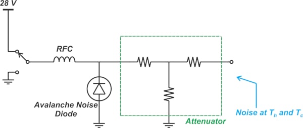
Figure 6. A simplified block diagram of a diode-based noise source.

 

When the 28 V supply is connected, the diode is reverse-biased into the avalanche region, producing a large amount of noise. On the other hand, when the supply is disconnected, only a small amount of noise appears at the output. The RF choke (RFC) is simply an inductor large enough to be considered an open circuit at all frequencies of interest. The attenuator helps us reduce the mismatch uncertainty. It ensures that no matter whether the diode is ON or OFF, the noise source exhibits a relatively constant, well-defined match at the output. While the physical temperature of a noise diode is room temperature, it can produce exceptionally “hot” noise levels. For example, in the range of 10,000 K, which is higher than the melting point of any known metal. The noise produced by modern noise sources is stable with time, has a broad frequency range, and exhibits a low reflection coefficient.  

 

The Excessive Noise Ratio Formula

Excessive noise ratio (ENR) is a common way to characterize the noise generated by active noise sources. ENR in decibels is defined as:

 

\[ENR (dB)=10 log \Big ( \frac{T_h - T_c}{T_0} \Big )\]

 

Where:

• T_h and T_c are the noise temperature of the noise source in its ON and OFF states
• T₀ is the reference temperature of 290 K

Note that the earlier definition of ENR was:

 

\[ENR (dB)=10 log \Big ( \frac{T_h - T_0}{T_0} \Big )\]

 

This definition was based on the assumption that T_c is equal to T₀. This is not usually the case in our measurements. However, the calibrated ENR values supplied by the noise source manufacturers are generally referenced to T₀ = 290 K. For example, if ENR is specified to be 15 dB, we have T_h = 9460.6 K. The most common ENR values for commercial noise sources are 5, 6, and 15 dB. There are also noise sources with higher ENR values, for example, 25 dB, but the availability of noise sources with ENR values above 15 dB is limited.

 

---

 

To see a complete list of my articles, please visit this page.