How to Design a Simple, Voltage-Controlled, Bidirectional Current Source

This article, part of AAC’s Analog Circuit Collection, presents a high-performance current source that requires only a few readily available components.

When all you’re doing is drawing a schematic, voltage sources and current sources are equally easy to implement. However, after we enter the real world of circuit design, we gradually realize that generating a more or less constant current is, for some reason, much more difficult than generating a more or less constant voltage. This doesn’t change the fact, though, that current sources are sometimes very useful, and it’s a good thing that clever engineers have created a variety of practical current-source circuits.

 

Current Source Recap

In this article, I want to share with you an interesting current source that I found in an old application note published by Linear Technology. First, though, I should mention other types of current sources that are discussed in existing AAC articles.

If you want to go down to the transistor level, we have articles on the MOSFET current mirror and the BJT current mirror. If you prefer to use operational amplifiers, the Howland current pump produces a voltage-controlled current and requires only one op-amp and four resistors.

 

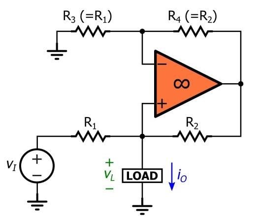
The Howland current pump.

 

If you don’t like working with discrete transistors and (for some reason) you don’t have any op-amps on hand, you might want to consider converting one of your linear voltage regulators into a current source.

The Jim Williams Current Source

This is by no means the official name for the circuit, and I certainly don’t want to imply that it’s the only current source that Jim Williams ever designed—I wouldn’t be surprised to learn that he came up with half a dozen innovative, high-performance current-source topologies. Nonetheless, he is the author of the app note and I don’t know what else to call the circuit.

As shown in the schematic below, this current source requires two amplifier ICs and a few passives.

 

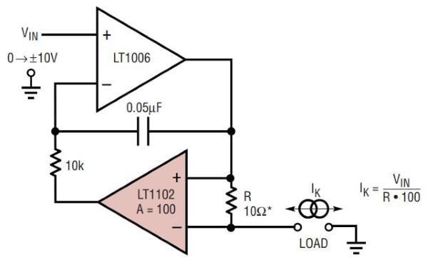
Diagram taken from the datasheet for the LT1102.

 

The LT1006 is a typical precision op-amp, and the LT1102 is a high-precision instrumentation amplifier. The application note was published in 1991, so these are some old ICs. I used the LT1006 and LT1102 in my simulation (which will be discussed in the next article) just to ensure that everything in the simulation is consistent with the original design—and, actually, Digi-Key still categorizes both of these parts as “active.” Nevertheless, I encourage you to experiment with some newer (and presumably higher-performance) replacements for these legacy ICs.

The following list highlights some of the characteristics of the Jim Williams current-source topology.

• It is voltage controlled and bidirectional—the magnitude and direction of the load current are determined by the magnitude and polarity of the input voltage.
• It is ground referenced; one side of the load resistance is connected directly to ground.
• As indicated by the equation included in the diagram above, the current magnitude is influenced also by R, that is, the value of the resistor placed between the input terminals of the instrumentation amplifier.
• If you use a very-high-precision resistor for R such that the error introduced by this component is negligible, the initial accuracy and temperature stability of the circuit correspond to the gain accuracy and temperature coefficient of the instrumentation amplifier.
• The circuit has good stability and is compatible with rapid changes in input voltage.

Understanding the Circuit

The key to the operation of this current source is the use of the instrumentation amplifier. By sensing the voltage across a fixed resistance that is in series with the load, we can generate an output current that is not influenced by the value of the load resistance.

Below is my attempt at a step-by-step explanation of how this circuit works.

 

 

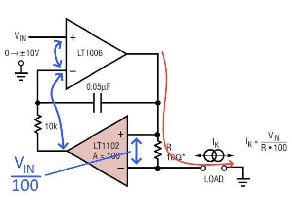
1. The op-amp (A1) is operating in a negative-feedback configuration. The presence of the instrumentation amplifier (A2) in the feedback path does not change the fact that the feedback loop has been closed.
2. The presence of negative feedback allows us to use the virtual short assumption. Thus, the output of A2 must be equal to the input voltage.
3. The virtual short condition doesn’t come out of nowhere; rather, the virtual short is imposed by the action of the op-amp’s output terminal. Since A2 has a gain of 100, A1’s output will do whatever is necessary to ensure that the voltage across R is equal to the input voltage divided by 100.
4. Since R is a fixed resistance, and since the voltage across R is always proportional to the input voltage, we know from Ohm’s law that the current through R will always be proportional to the input voltage.
5. Since the load is in series with the resistor R, the output current is always proportional to the input voltage, regardless of the load resistance (within limits, of course—e.g., you won’t be able to drive 10 mA through a 1 MΩ load unless you can find amplifiers that accept supply voltages up to 10,000 V or so).
6. The capacitor and the other resistor determine the circuit’s frequency response, and I assume that the values have been chosen so as to create a desirable phase margin.

 

Conclusion

We’ve looked at a straightforward bidirectional-current-source topology that is built around a high-precision operational amplifier and a high-precision instrumentation amplifier.

In the next article, we’ll use some LTspice simulations to further explore the operation and performance of this circuit.