Facebook
 Google
 GitHub
 Linkedin
Temperature Drift in Resistors and Op-amps—Flicker Noise and Signal Averaging
Learn about temperature drift in electronic circuits, namely in resistors and amplifiers. We'll also cover how the effect of flicker noise comes into play and how drift limits the effectiveness of signal averaging.
Even under fixed electrical conditions (supply voltage, input, and load), electronic circuits are not perfectly stable as they tend to drift with time and temperature. These deviations from the ideal behavior can add a considerable error to precision measurements. To gain insight into temperature drift in electronics, this article briefly looks at the temperature behavior of resistors and amplifiers. We’ll also discuss that the effect of the flicker noise might not be easily distinguishable from a temperature-induced drift in the output. Finally, we’ll discuss that drift can limit the effectiveness of the signal averaging technique that is commonly used to increase the accuracy of repeatable measurements.
Resistor Temperature Drift—Resistor Temperature Coefficient
Being perhaps the simplest type of electronic component, resistors might be overlooked as error sources in high-performance circuits. However, the value of a resistor is not constant and changes with temperature and time. As an example, if the temperature coefficient of a resistor is ±50 ppm/°C and the ambient temperature goes 100 °C above the reference temperature (the room temperature), the value of the resistor can change by ±0.5 %.
Luckily, in many applications, the circuit accuracy is determined by the ratio of two or more resistors rather than the absolute value of a single resistor. In these cases, a matched resistor network, such as the LT5400, can be used. The resistors form a common-substrate network and exhibit well-matched temperature behavior. Figure 1 compares the temperature behavior of a single discrete resistor with that of a matched resistor network.
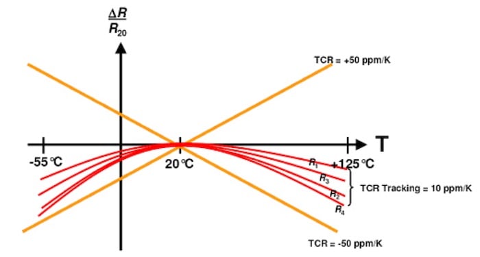
Figure 1. A discrete resistor of a matched resistor network's temperature behavior. Image used courtesy of Vishay
In this figure, the orange lines specify the limits for the change in the value of a single ±50 ppm/°C resistor as the temperature changes in either direction from the reference temperature (20°C). The red curves correspond to four resistors from a matched resistor network that exhibit similar temperature behavior. Temperature coefficients (TC) of the matched resistors track one another, typically to within 2–10 ppm/°C. Resistors with well-matched temperature behavior can be a fundamental requirement in certain precision applications such as resistive current sensing.
Temperature-induced Drift With an Identical Temperature Coefficient
It should be noted that, even with identical TC values, the resistors in a circuit can generate a temperature-dependent drift. Below you can see an example in Figure 2.
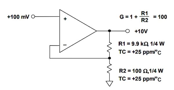
Figure 2. An example where temperature-dependent drift is created. Image [modified] used courtesy of Analog Devices
In the above figure, the two resistors have identical TCs (+25 ppm/°C); however, the voltage across the resistors and, consequently, the power dissipated by the two resistors is very different. The voltage across R2 = 100 Ω is 0.1 V, which leads to a power dissipation of 0.1 mW. However, the voltage across R1 is 9.9 V; thus 9.9 mW is dissipated across this resistor. Assuming that the thermal resistance of both resistors is 125 °C/W, the temperature of R1 and R2 will respectively rise by 1.24 °C and 0.0125 °C above the ambient temperature. This unequal self-heating effect causes the two resistors to drift by different amounts.
Figure 3(a) shows another example where identical TCs cannot necessarily resolve the temperature drift issue.
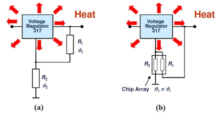
Figure 3. An example using (a) discrete resistors for different local ambient temperatures and (b) using integrated resistors/resistor arrays for equal local ambient temperatures. Image used courtesy of Vishay
In the above figure, if the design incorporates unequal resistors (R1 ≠ R2) with identical TCs, the self-heating of the resistors can generate a temperature-induced drift as we discussed above. However, an additional temperature gradient can be caused by the voltage regulator. This temperature gradient generates unequal temperature drifts in the resistors even if the resistance and TC of the two resistors are the same (R1 = R2 and TC1 = TC2).
A resistor array can be used to avoid the drift issue of the above examples (Figure 3(b)). With a resistor network implemented on a single substrate, the two resistors are thermally coupled and experience the same ambient temperature.
Temperature Drift in Other Circuits—Op-amp Temperature Drift
With a simple resistor being susceptible to temperature and aging, it is not surprising that the parameters of other more complex circuits also drift with temperature and time. For example, the input offset voltage of an amplifier changes with temperature and time. This can produce a time-varying error, limiting the minimum DC signal that can be measured. The offset drift for a typical general purpose precision op-amp can be in the range of 1–10 μV/°C.
If the offset drift of an amplifier limits the accuracy of our measurements, we can consider the use of a chopper-stabilized amplifier. These devices use offset cancellation techniques to reduce the offset voltage to a very low level (e.g., less than 10 μV) and yield a near zero-drift operation. The offset drift of a chopper-stabilized amplifier, such as the MCP6V51 from Microchip, can be as low as 36 nV/°C.
Temperature Drift or Flicker Noise (1/f)?
At very low frequencies, the flicker noise is the dominant noise source that affects the output of a circuit. The average power of the flicker noise is inversely proportional to the frequency of operation (that’s why the flicker noise is also called 1/f noise). The lower the frequency, the higher the average power of the 1/f noise. If we measure the output of a circuit for a sufficiently long time, we can capture the effect of this low-frequency noise. Figure 4 shows the amplified fluctuations the flicker noise produces at the output of the ADA4622-2.
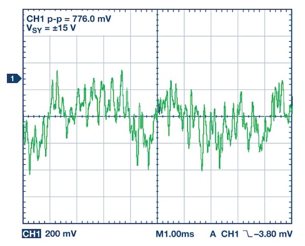
Figure 4. The amplified fluctuations from the flicker noise of the ADA4622-2's output. Image used courtesy of Analog Devices
The ADA4622-2 is a precision op-amp with a 0.1 Hz to 10 Hz noise of 0.75 μV p-p typical. The figure above's waveform shows the 0.1 Hz to 10 Hz noise of the ADA4622-2 amplified by a factor of 1000. As you can see, the flicker noise causes random slow fluctuations in the output. These fluctuations are produced by a phenomenon different from the temperature- or aging-induced drift. However, due to its low-frequency nature, the effect of the 1/f noise might not be easily distinguishable from a drift in the signal.
In the case of op-amps, both offset drift and 1/f noise cause slow errors at the output. That’s why a zero-drift op-amp, which uses offset cancellation techniques to reduce the offset drift, doesn’t have 1/f noise at the output. Figure 5 compares the 1/f noise of a continuous-time amplifier with that of a zero-drift amplifier.
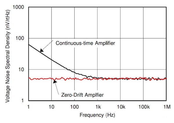
Figure 5. The noise of a continuous-time amplifier vs a zero-drift amplifier. Image used courtesy of TI
Drift Can Limit the Effectiveness of Signal Averaging?
Another effective noise reduction technique is signal averaging. If we have a repeatable experiment with a noise variance of $$σ_n^2$$, we can repeat the experiment M times and average the corresponding output samples to reduce the noise variance to:
$$σ_{n, avg}^2 = \frac{σ_n^2}{M}$$
Equation 1.
Where $$σ_{n, avg}^2$$ denotes the noise variance of the averaged signal. Despite signal averaging's effectiveness in certain applications, it still has its limitations. Signal averaging is based on the assumption that the noise samples are not correlated with each other. A slow drift in the measured data can act as a low-frequency correlated noise component and limit the effectiveness of the signal averaging technique. In this case, the noise suppression will be lower than that predicted by Equation 1. Additionally, depending on the type of the random drift in a given application, the variance of the averaged signal can increase above certain values of M.
In another article, we’ll examine this limitation of the signal averaging technique more closely and introduce a useful statistical analysis tool, called Allan variance, that allows us to have a deeper insight into how the output of a circuit tends to drift due to different phenomena such as the flicker noise, temperature effect, etc.
To see a complete list of my articles, please visit this page.
Related Content