Facebook
 Google
 GitHub
 Linkedin
What Is Dynamic Range?
The concept of dynamic range appears frequently in engineering discussions. But what exactly does this term mean? And how does it apply to electronic circuits and systems?
An interesting phenomenon of language is that we often understand words that we cannot define. This is part of our natural linguistic faculty and usually doesn’t cause any problems, especially in ordinary conversation.
In the world of engineering, though, we place greater emphasis on precision and clarity. Discussing technical details, mathematical relationships, and performance specifications is not always easy, and we can make the task more manageable and productive by striving to carefully employ and thoroughly understand the relevant terminology.
One term that electrical engineers confront regularly, and in a variety of contexts, is “dynamic range.” Before you continue reading, take a minute and try to formulate a precise, comprehensive definition. In my opinion, it’s surprisingly difficult! In any case, I hope that by the end of this article we’ll all be ready with a solid explanation when someone stops us on the street and asks, “Hey, could you tell me what dynamic range is?”
Static vs. Dynamic Range
As far as I know, the term “static range” doesn’t exist. But let’s pretend that it does and use it to clarify the nature of dynamic range.
“Range” is defined as the region of variation between two limits. “Static,” from a Greek verb related to standing or motionlessness, denotes a lack of movement, action, or change. Thus, static range suggests a region of possible variation in which the limits are not constrained by the need for input or output phenomena to actively and unpredictably move between the upper and lower limits.
“Dynamic”—essentially the opposite of “static”—describes that which is continuously moving and changing. With dynamic range, we still have upper and lower limits, but these limits apply to systems that are constrained by the continuous variation of input or output phenomena, and they capture the capabilities of the system with respect to operating conditions that reflect the dynamic nature of the relevant signals.
With the foregoing information in mind, we can say that dynamic range, in the context of electrical engineering, specifies the range of possible or acceptable values that a dynamic signal can assume when delivered to or produced by a given system.

Case in Point: Human Vision
Let’s consider an example. The human visual system has a remarkable capacity for variations in input magnitude. We can see ripples on a moonlit pond and a white sail gleaming under a blinding Mediterranean sun. The luminance range to which the human eye is sensitive spans fourteen orders of magnitude: the lower limit is about 10–6 candelas per square meter (cd/m2), and the upper limit is about 108 cd/m2.
Does this mean that the human visual system has a dynamic range of 1014? No, because the luminance range mentioned above includes the sensitivity of both cone and rod cells, and these two biological photoreceptors don’t provide simultaneous operation (the system actually needs a significant amount of time to transition from its high-luminance mode to its low-luminance mode). Thus, the range doesn’t apply to input signals that are dynamically varying between upper limit and lower limit and thereby restricting the system to a certain set of operating conditions.
To determine the dynamic range of human light detection, we need to evaluate our ability to perceive a range of luminance while looking steadily at one scene. If we apply a stricter interpretation of dynamic range, we would not allow changes in pupil size, since this is analogous to moving the upper or lower limit by increasing or decreasing gain.
Calculating and Expressing Dynamic Range
A dynamic range is really just a ratio: you take the maximum signal level and divide it by the minimum signal level.
Electrical engineers tend to use decibels to express large ratios (such as the gain of an op-amp), and dynamic range is no exception. If a voltage-monitoring system, for example, has a dynamic range of 80 dB, the maximum detectable input level is greater than the minimum detectable input level by a factor of 10,000.
In optical systems, dynamic range is often expressed in stops. One stop is a factor-of-two increase or decrease. If we say that a digital camera has a dynamic range of 8 stops, it can faithfully reproduce a scene if the luminance of the brightest portion divided by the luminance of the darkest portion is less than or equal to 256 (=28).

The dB values are rounded to one decimal place, and the stop values are rounded to the nearest third stop.
Dynamic Range in Electronic Systems
The following subsections provide examples of dynamic range in different types of circuits.
Analog-to-Digital Converters
If we’re thinking in terms of output, the dynamic range of an ADC is determined by the resolution. The lowest non-zero output value is 1, and the highest output value is (2N–1), where N is the number of bits in the generated digital word. Thus, a 14-bit ADC has a dynamic output range of (214–1) =16383. This could also be expressed as 84.3 dB or 14 stops.
The dynamic range of the input signal is less straightforward, because the lower limit is determined by the amount of noise in the analog waveform, which could be influenced by environmental conditions or the gain setting of a variable-gain amplifier that precedes the ADC. If the reference voltage imposes an upper limit of 2.5 V and the noise floor is 1 mV, the dynamic range is 2.5/1×10–3 ≈ 68 dB.
You can read much more about ADC dynamic range in the following articles:
- Understanding the Dynamic Range Specification of an ADC
- Assessing the ADC SNR and SFDR for Communications Systems

A specialized type of dynamic range called spurious-free dynamic range (SFDR) can be used to quantify the linearity of a circuit.
Image Sensors
In a CCD sensor, the upper limit on optical detection is the number of light-generated electrons that can be stored in a pixel, and the lower limit is the number of electrons associated with dark noise and read noise. Let’s say that a pixel can hold 40,000 electrons. If in a given exposure period the pixel generates 5 electrons of dark noise and receives an additional 10 electrons of noise during readout, the dynamic range is 40,000/(5+10) = 68.5 dB or about 11⅓ stops.
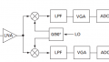
RF Mixers
Mixers perform frequency translation and therefore play a fundamental role in the design of radio-frequency systems. The input power level at which the mixer begins to exhibit unacceptable nonlinearity is called the 1 dB compression point. This corresponds to the upper limit used in calculating the dynamic range, and the lower limit is the mixer’s noise figure.
Conclusion
This article was more difficult to write than I expected. I hope that I’ve done enough to really capture the essence and subtleties of dynamic range as it pertains to electrical engineering, and if you have any insights to add, feel free to share them in the comments section.