 Facebook
 Google
 GitHub
 Linkedin
Node Voltage Method
What is the Node Voltage Method for DC Network Analysis?
The node voltage method is a DC network analysis technique based on the structured application of Kirchhoff’s current law. This method involves converting voltage sources to current sources and replacing resistances with equivalent conductances.
The node voltage method of DC network analysis solves for unknown voltages at circuit nodes in terms of a system of Kirchhoff’s current law (KCL) equations. This analysis looks strange because it replaces voltage sources with equivalent current sources. Additionally, resistor values in ohms are replaced by equivalent conductances (G = 1/R) with units of siemens (S). Once understood, the node voltage method can provide a simple technique for quickly solving various complex circuits.
In this textbook page, we will demonstrate the node voltage method on two circuits, including an unbalanced Wheatstone bridge.
Node Voltage Method Steps
First, let’s start with a circuit having conventional voltage sources, as illustrated in Figure 1.
Step 1: Label All Unique Voltage Nodes
A common node, V0, is chosen as a reference point—this is typically the ground node in the circuit. The other unknown node voltages in our Figure 1 circuit, V1 and V2, will be calculated concerning this point.

Figure 1. Circuit schematic for demonstration of the node voltage method of circuit analysis.
Step 2: Replace All Voltage Sources and Series Resistors With Current Sources and Parallel Resistors
Next, we need to replace all voltage sources and their associated series resistors with equivalent current sources and parallel resistors. The current source value is calculated as:
$$I_{source} = \frac{V_{source}}{R_{series}}$$
The voltage source, B1, in Figure 1 is in series with resistor, R1, which has a current source value of 5 A:
$$I_1 = \frac{V_{B1}}{R_1} = \frac{10 \text{ V}}{2 \text{ }\Omega} = 5 \text{ A}$$
The parallel resistance will be the same value as the series resistance. Knowing our current source and resistance values, we can draw our equivalent parallel circuit, as shown in Figure 2.
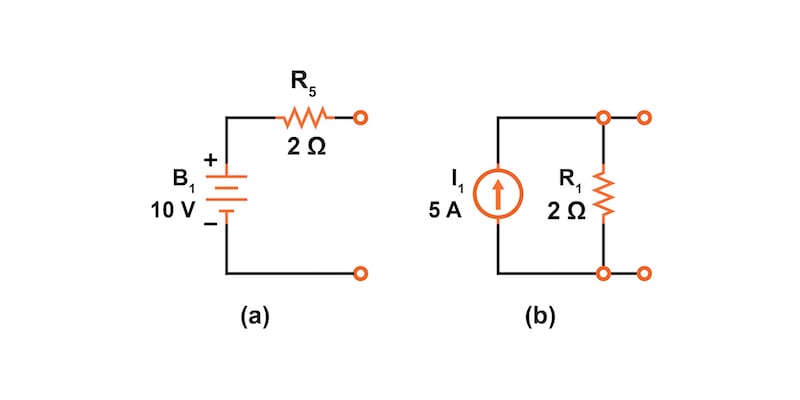
Figure 2. Conversion of a voltage source with series resistance to a current source with parallel resistance.
We need to perform the same voltage source to current source conversion for battery, B2, with a series resistor, R5, from our circuit in Figure 1.
$$I_2 = \frac{V_{B2}}{R_5} = \frac{-4 \text{ V}}{1 \text{ }\Omega} = -4 \text{ A}$$
From here, we can now redraw our circuit with two current sources and parallel resistors, as shown in Figure 3.
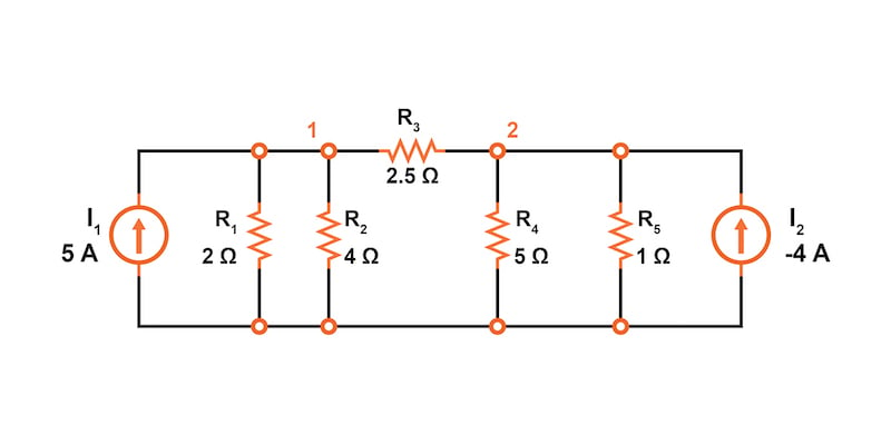
Figure 3. New circuit with current sources and parallel resistors.
Step 3: Replace Resistor Resistance in Ohms with Conductance in Siemens
For all resistors in our circuit, we must now replace the resistance value in ohms with its reciprocal conductance value in siemens. The siemens is the unit of conductance, having replaced the now obsolete mho (inverse of an ohm) unit.
$$G_1 = \frac{1}{R_1} = \frac{1}{2 \text{ }\Omega} = 0.5 \text{ S}$$
$$G_2 = \frac{1}{R_2} = \frac{1}{4 \text{ }\Omega} = 0.25 \text{ S}$$
$$G_3 = \frac{1}{R_3} = \frac{1}{2.5 \text{ }\Omega} = 0.4 \text{ S}$$
$$G_4 = \frac{1}{R_4} = \frac{1}{5 \text{ }\Omega} = 0.2 \text{ S}$$
$$G_5 = \frac{1}{R_4} = \frac{1}{1 \text{ }\Omega} = 1 \text{ S}$$
We can update our drawing with these calculated conductance values (Figure 4).
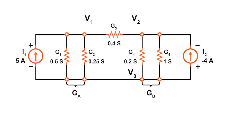
Figure 4. All resistance values are replaced by equivalent conductance.
At this point, we can also simplify the circuit by combining parallel conductors. We do this by simple addition. In our circuit of Figure 4, we have two sets of parallel conductors:
$$G_A = G_1 + G_2 = 0.5 + 0.25 = 0.75 \text{ S}$$
$$G_B = G_4 + G_5 = 0.2 + 1 = 1.2 \text{ S}$$
Our simplified circuit, ready for applying the node voltage method, is shown in Figure 5.
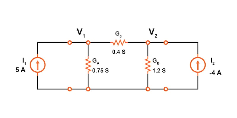
Figure 5. Simplified circuit.
Step 4: Write KCL Equations for Each Unknown Voltage Node
Following the node voltage method, we now write KCL equations for all unknown voltage nodes. In our example circuit, we have only two unknown node voltages, V1 and V2.
$$I_1 = G_AV_1 + G_3(V_1-V_2)$$
Equation 1.
$$I_2 = G_BV_2 + G_3(V_2-V_1)$$
Equation 2.
Let’s rewrite these two equations to demonstrate a pattern for writing these equations by inspection.
$$I_1 = (G_A + G_3)V_1 - G_3V_2$$
Equation 1.
$$I_2 = (G_B + G_3)V_2 - G_3V_1$$
Equation 2.
Note the similarity in these two equations. The sum of conductances connected to the first KCL node (GA + G3) is the positive coefficient of the first voltage (V1) at that node in Equation 1. Likewise, in Equation 2, the sum of conductances connected to that KCL node for V2 is the positive coefficient of the voltage, V2, in Equation 2. The other coefficients are negative, representing conductances between other non-common nodes.
For both equations, the left-hand side is equal to the respective current source connected to the node. This pattern allows us to quickly write the equations by inspection. If you can learn this relatively simple pattern for writing the KCL equations using conductances, the node voltage method can be useful for quickly analyzing many circuits.
Step 5: Solve the Set of Simultaneous KCL Equations for the Unknown Voltages
From here, we can use the two equations to solve for the two unknown voltages in our circuit. We can substitute our known currents and conductances and rearrange them to order like terms.
$$I_1 = 5 = (0.75 + 0.4)V_1 - 0.4V_2 = 1.15V_1 - 0.4V_2$$
$$I_2 = -4 = (1.2 + 0.4)V_2 - 0.4V_1 = -0.4V_1 + 1.6V_2$$
Solving these simultaneous equations, we get the following results for our node voltages:
$$V_1 = 3.8095 \text{ V}$$
$$V_2 = -1.5476 \text{ V}$$
Verification of the Node Voltage Method Using SPICE
The solution can then be verified using SPICE based on the original schematic diagram with voltage sources. However, the circuit with the current sources could also have been simulated.
           * Node Voltage Method circuit simulation
           V1 11 0 DC 10
           V2 22 0 DC -4
           r1 11 1 2
           r2 1 0 4
           r3 1 2 2.5
           r4 2 0 5
           r5 2 22 1
           .DC V1 10 10 1 V2 -4 -4 1
           .print DC V(1) V(2)
           .end

                v(1)            v(2)
            3.809524e+00    -1.547619e+00
The Node Voltage Method Applied to an Unbalanced Wheatstone Bridge
Let’s look at another circuit analysis example using the node voltage method. The circuit of Figure 6 is called an unbalanced Wheatstone bridge, and it has three unknown voltage nodes plus the common voltage node, V0.
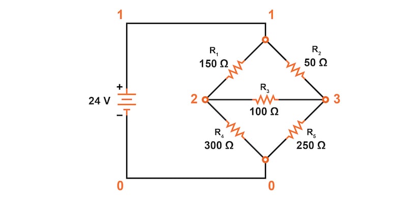
Figure 6. Wheatstone bridge for node voltage method application.
It’s important to note that we do not list the conductances on the schematic diagram. However, G1 = 1/R1, etc.
There are three nodes (V1, V2, and V3) to write equations for by inspection. Remember, the conductance coefficients are positive for conductors connected to the node we are developing the KCL equation for. All other conductance coefficients are negative.
Since we are too lazy to calculate the conductances for the resistors on the diagram, the subscripted G’s are listed for now as the coefficients.
$$I_1 = 0.136092 = (G_1+G_2)V_1 - G_1V_2 -G_2V_3$$
$$I_2 = 0 = (G_1 + G_3 + G_4)V_2 - G_1V_1 - G_3V_3 $$
$$I_3 = 0 = (G_2 + G_3 + G_5)V_3 - G_2V_1 - G_3V_2 $$
Next, we can reorder to align the unknown voltages to make it easier to solve the simultaneous equations:
$$0.136092 = (G_1+G_2)V_1 - G_1V_2 -G_2V_3$$
$$0 = - G_1V_1 + (G_1 + G_3 + G_4)V_2 - G_3V_3 $$
$$0 = - G_2V_1 - G_3V_2 + (G_2 + G_3 + G_5) $$
Again, we are so lazy that we will solve this using GNU Octave and enter reciprocal resistances and sums of reciprocal resistances into the Octave “A” matrix, letting Octave compute the matrix of conductances after “A =.”
The initial entry line was so long that it was split into three rows. The entered “A” matrix is delineated by starting and ending square brackets. Column elements are space-separated. Rows are “new line” separated. Commas and semicolons are not needed as separators. Though, the current vector at “b” is semicolon-separated to yield a column vector of currents.
octave:12> A = [1/150+1/50 -1/150 -1/50
           > -1/150 1/150+1/100+1/300 -1/100
           > -1/50 -1/100 1/50+1/100+1/250]
           A =
              0.0266667  -0.0066667  -0.0200000
             -0.0066667   0.0200000  -0.0100000
             -0.0200000  -0.0100000   0.0340000

           octave:13> b = [0.136092;0;0]
           b =
              0.13609
              0.00000
              0.00000

           octave:14> x=A\b
           x =
              24.000
              17.655
              19.310
Note that the diagonal coefficients in the “A” matrix are positive, while the other coefficients are all negative, as they must be based on our rules for writing the node voltage method equations.
The voltage vector solution is given in “x”:
- V1 = 24.000 V
- V2 = 17.655 V
- V3 = 19.310 V
These three voltages are identical to the results we obtained using the mesh current analysis and SPICE simulation of the unbalanced Wheatstone bridge. This is no coincidence, for the 0.13609 A current source was purposely chosen to yield the 24 V used as a voltage source in that problem.
Review of the Node Voltage Method
- The node voltage method is a circuit analysis technique based on the structured application of Kirchhoff’s current law after replacing all voltage sources with current sources and replacing resistances with conductances.
- The node voltage method follows a 5-step process:
- Step 1: Label all unique voltage nodes after selecting a reference node (typically ground)
- Step 2: Replace all voltage sources and series resistors with current sources and parallel resistors
- Step 3: Replace resistor resistance in ohms with conductances in siemens
- Step 4: Write KCL equations for each unknown voltage node
- Step 5: Solve the set of simultaneous KCL equations for the unknown voltages
- When writing the KCL equations in Step 4, it is possible to write these by inspection.
- The positive coefficient of the first voltage in the first equation is the sum of conductances connected to the node. The coefficient for the second voltage in the second equation is the sum of conductances connected to that node. Repeat for the coefficient of the third voltage, third equation, and other equations.
- All other coefficients for all equations are negative, representing conductances from the voltage node under KCL evaluation to all other nodes. In the first equation, the second coefficient is the conductance from node 1 to node 2, the third coefficient is the conductance from node 1 to node 3. Fill in negative coefficients for other equations.
- The other side of these KCL equations is the current source connected to the respective nodes.
Related Content
Below you’ll find additional resources to learn more about the node voltage method and related analysis:
Calculators:
Worksheets:
- Precise Diode Circuits Worksheet
- Kirchhoff’s Laws Worksheet
- DC Bridge Circuits Worksheet
- AC Network Analysis Worksheet
Video Tutorials and Lectures:
Technical Articles:


Brrrrrrrrrrrruh you saved my ass
This is very helpful and well explained!
Hello, formatting is broken on some of the equations.