Solving Unbalanced Wheatstone Bridge Circuits Via Mesh Current Method

An unbalanced Wheatstone bridge cannot be solved using simple series and parallel circuit analysis because the resistors are connected in a complex configuration. This section provides a step-by-step walkthrough demonstrating how to solve an unbalanced Wheatstone bridge using the mesh current method (also known as the loop current method). 

 

Unbalanced Wheatstone Bridge

First, let’s determine the voltages and currents for the unbalanced Wheatstone bridge circuit of Figure 1.

 

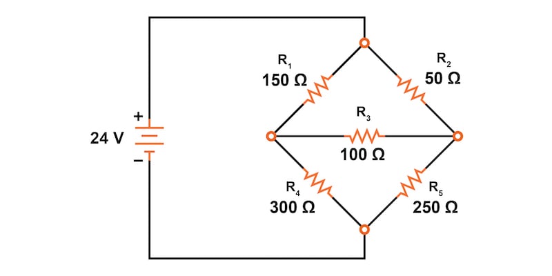
Figure 1. Unbalanced Wheatstone bridge circuit schematic.

 

Since the ratios of R₁ / R₄ and R₂ / R₅ are not equal, there will be a voltage across the resistor, R₃, and some amount of current through it. As discussed at the beginning of this chapter on network analysis theorems, this type of circuit is irreducible by normal series-parallel analysis and may only be analyzed by some other method.

We could apply the branch current method to this circuit, but it would require six currents (I₁ through I₆), leading to a large set of simultaneous equations to solve. On the other hand, using the mesh current method, we may solve for all currents and voltages with fewer variables.

Below are the six steps of the mesh current method:

1. Identify and label the current loops
2. Label the voltage drop polarities
3. Apply Kirchhoff’s voltage law (KVL) to each loop
4. Solve the simultaneous equations for the unknown currents
5. Redraw the mesh currents and determine the branch currents
6. Calculate the voltage drops using Ohm’s law

 

Step 1: Identify and Label the Current Loops

The first step in the mesh current method is to draw just enough mesh currents to account for all components in the circuit. Looking at our bridge circuit, it should be obvious where to place two of these current loops, as shown in Figure 2.

 

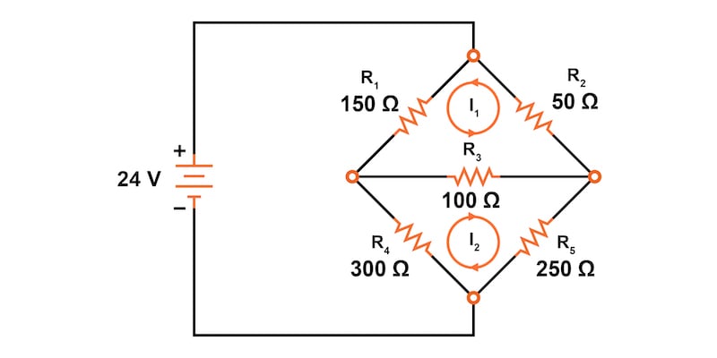
Figure 2. Current loops 1 and 2 were added to the Wheatstone bridge circuit.

 

The directions of these mesh currents, of course, are arbitrary. However, two mesh currents are insufficient in this circuit because neither I₁ nor I₂ go through the battery. Thus, we must add a third mesh current, I₃, as illustrated in Figure 3.

 

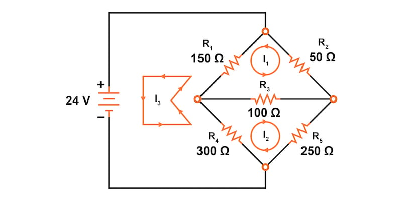
Figure 3. Current loop 3 added to the Wheatstone bridge circuit.

 

Here, we’ve chosen I₃ to loop from the negative terminal of the battery, through R₄ through R₁, and back to the positive terminal of the battery. This is one of many paths that could have been chosen for I₃, but this example seems the simplest.

 

Step 2: Label the Voltage Drop Polarities

Now, we must label the resistor voltage drop polarities, following each current direction (Figure 4).

 

Figure 4. Label the voltage drop polarities.

 

Step 3: Apply Kirchhoff’s Voltage Law to Each Loop

Next, let’s generate a KVL equation for the top loop of the bridge, starting from the top node and tracing it in a clockwise direction. This results in the following equations:

 

$$R_2I_1 + R_3(I_1 + I_2) + R_1(I_1 - I_3) = = 0 \text{ V}$$

 

$$50I_1 +100(I_1 + I_2) + 150(I_1 - I_3) = 0 \text{ V}$$

 

In this equation, we represent the current through each resistor as the algebraic sum of the loop currents. For example, resistor R₃ has its voltage represented in the above KVL equation by the expression 100(I₁ + I₂) since both currents, I₁ and I₂, go through R₃ in the same direction. The voltage across resistor R₁ is expressed as 150(I₁ - I₃) since loop currents I₁ and I₃ oppose each other. 

Combining like terms, we can simplify this to:

 

$$300I_1 +100I_2 - 150I_3 = 0 \text{ V}$$

 

Now, we can repeat that same process to generate a KVL equation for the bottom loop of the Wheatstone bridge. Let’s start at the bottom and move counterclockwise. 

 

$$R_5I_2 + R_3(I_2+I_1) + R_4(I_2+I_3) = = 0 \text{ V}$$

 

$$250I_2 + 100(I_2+I_1) + 300(I_2+I_3) =0 \text{ V}$$

 

After combining like terms, we get the following equation:

 

$$100I_1 + 650I_2 + 300I_3 =0 \text{ V}$$

 

Note how the second term in the equation’s original form has resistor R₃‘s value of 100 Ω multiplied by the sum of I₂ and I₁ (I₂ + I₁) because those currents flow in the same direction through R₃. The same applies to currents I₂ and I₃ passing through resistor R₄.

With that done, we’ve now taken care of two equations; however, we still need a third equation to complete the simultaneous equation set of three variables and three equations. This third equation must also include the battery’s voltage, which up to this point, does not appear in either two of the previous KVL equations. 

To generate this equation, we will trace a loop again with our imaginary voltmeter starting from the battery’s bottom (negative) terminal, stepping clockwise. Again, the direction in which we step is arbitrary and does not need to be the same as the direction of the mesh current in that loop.

 

$$24 + R_1(I_3 - I_1) + R_4(I_3 + I_2) = = 0 \text{ V}$$

 

$$24 + 150(I_3 - I_1) + 300(I_3 + I_2) = 0 \text{ V}$$

 

Again, combining like terms and simplifying the equation, we get:

 

$$-150I_1 + 300I_2 + 450I_3 = 24 \text{ V}$$

 

Step 4: Solve the Simultaneous Equations for Unknown Currents

Now we have three simultaneous equations that we can solve using any method we prefer:

 

$$300I_1 +100I_2 - 150I_3 = 0 \text{ V}$$

KVL of Loop 1

 

$$100I_1 + 650I_2 + 300I_3 =0 \text{ V}$$

KVL of Loop 2

 

$$-150I_1 + 300I_2 + 450I_3 = 24 \text{ V}$$

KVL of Loop 3

 

First off, we will use GNU Octave, an open-source Matlab clone, to solve these equations. We can enter the resistor coefficients into a matrix, A, between square brackets with column elements separated by commas and rows separated by semicolons. 

Next, we can enter the voltages into a column vector, b. The unknown currents: I₁, I₂, and I₃ are calculated by the command: x = A \ b. These currents are contained within the resulting x-column vector.

 
octave:1>A = [300,100,150;100,650,-300;-150,300,-450]
        A =
          300  100  150
          100  650  -300
          -150 300  -450
 
        octave:2> b = [0;0;-24]
        b =
          0
          0
          -24
               
        octave:3> x = A\b
        x =
          -0.093793
           0.077241
           0.136092
 

Therefore the values of our loop currents are:

• I₁ = -93.793 mA
• I₂ = 77.241 mA
• I₃ = -136.092 mA

 

Step 5: Redraw the Mesh Currents and Determine the Branch Currents

The negative values for currents I₁ and I₃ indicate that our assumed current directions were in the wrong direction. For I₃, it makes intuitive sense because the current would have to flow out of the only power source in our circuit.

Thus, the actual loop current directions and the directions resistor are shown in Figure 5.

 

Figure 5. Correcting the loop current directions and determining the branch resistor currents.

 

From here, we can calculate the branch resistor current values:

 

$$I_{R1} = I_3 - I_1 = 136.092 - 93.793 = 42.299 \text{ mA}$$

 

$$I_{R2} = I_1 = 93.793 \text{ mA}$$

 

$$I_{R3} = I_1 - I_2 = 93.793 - 77.241 = 16.552 \text{ mA}$$

 

$$I_{R4} = I_3 - I_2 = 136.092 - 77.241 = 58.851 \text{ mA}$$

 

$$I_{R5} = I_2 = 77.241 \text{ mA}$$

 

Step 6: Calculate the Voltage Drops

Finally, we can calculate the voltage drops across each resistor:

 

$$V_{R1} = I_{R1}R_1 = (0.042299) \cdot (150) = 6.3448 \text{ V}$$

 

$$V_{R2} = I_{R2}R_5 = (0.093793) \cdot (50) = 4.6897 \text{ V}$$

 

$$V_{R3} = I_{R3}R_5 = (0.016552) \cdot (100) = 1.6552 \text{ V}$$

 

$$V_{R4} = I_{R4}R_5 = (0.058851) \cdot (300) = 17.6553 \text{ V}$$

 

$$V_{R5} = I_{R5}R_5 = (0.077241) \cdot (250) = 19.3103 \text{ V}$$

 

Using SPICE to Verify Our Voltage Calculations

Next, to confirm the accuracy of our voltage calculations, we can use a SPICE simulation using the circuit of Figure 6.

 

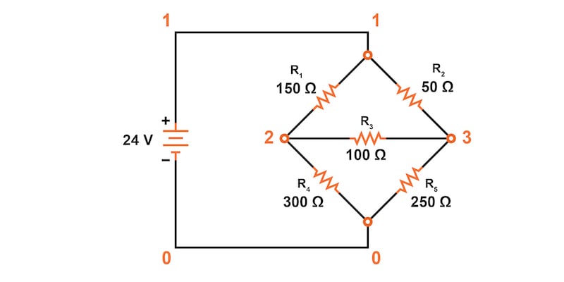
Figure 6. Node number labeling for SPICE simulation.

 

unbalanced wheatstone bridge  
v1 1 0 
r1 1 2 150     
r2 1 3 50      
r3 2 3 100     
r4 2 0 300     
r5 3 0 250     
.dc v1 24 24 1 
.print dc v(1,2) v(1,3) v(3,2) v(2,0) v(3,0)   
.end
v1          v(1,2)     v(1,3)      v(3,2)     v(2)       v(3)           
2.400E+01   6.345E+00  4.690E+00   1.655E+00  1.766E+01  1.931E+01

 

Mesh Current Method for an Unbalanced Wheatstone Bridge Review

Using the mesh current method, we were able to solve for the currents and voltages in an unbalanced Wheatstone bridge. The three simultaneous KVL equations with three unknown loop currents were solved using GNU Octave. We then validated our results using SPICE circuit simulation software.

 

Related Content

Below you can find additional resources concerning mesh current analysis and Wheatstone bridge circuits:

 

Calculators:

• Wheatstone Bridge Calculator
• Ohm's Law Calculator
• Parallel Resistor Calculator

 

Worksheets:

• DC Bridge Circuit Worksheet
• DC Mesh Current Analysis Worksheet
• AC Network Analysis Worksheet
• Ohm's Law Worksheet
• Kirchhoff's Laws Worksheet

 

Video Tutorials and Lectures:

• Complex Circuits
• Series-parallel Circuits
• Troubleshooting Series-parallel Circuits
   

Technical Articles:

• Mesh Analysis and Dependent Sources