Dynamic Nonlinearity in RF Power Amplifiers: Insights From Two-Tone Testing

Multiple mechanisms contribute to dynamic nonlinearity in power amplifiers (PAs). For example, the third-order intermodulation (IM3) distortion produced by a PA varies with—among other factors—the input amplitude and signal bandwidth. Earlier in this series of articles, we used a two-tone input test to help us understand intermodulation distortion in RF systems. Now, we’ll examine how the frequency separation of the two tones during testing can lead to dynamic nonlinearity in RF PAs.

For this discussion, it’s essential that we comprehend both the distortion generated by a single-stage nonlinear amplifier and the distortion generated by a cascaded system of amplifiers. We’ll pay particular attention to the mixing mechanisms that produce IM3 components in cascaded stages. Let’s start, however, by reviewing the distortion products of a single-stage amplifier.

 

Applying a Two-Tone Input to a Single-Stage Amplifier

Consider the following two-tone input, which comprises frequency components at ⍵₁ and ⍵₂:

$$x(t) ~=~ A_1 \cos(\omega_1 t) ~+~A_2 \cos(\omega_2 t)$$

Equation 1.

 

If we introduce this two-tone input to a nonlinear system represented by the following polynomial expression:

$$y(t) \approx \alpha_0 ~+~ \alpha_1 x(t) ~+~ \alpha_2 x^2(t) ~+~ \alpha_3 x^3(t)$$

Equation 2.

 

then several different distortion products will emerge at the output. Figure 1 illustrates the complete range of distortion products generated by this third-degree expression.

 

Figure 1. Frequency components produced by the linear term (green), the second-order term (blue), and the third-order term (orange) when the input-output characteristic is modeled by a third-degree expression. Image used courtesy of Steve Arar

 

In the above figure, the green components represent the desired outputs produced by the linear term (⍺₁). The blue and orange components are generated by the second-order term (⍺₂) and the third-order term (⍺₃), respectively. As in previous articles, note that the figure is not meant to accurately represent the magnitude of the signal components. It shows only their presence and the frequencies at which they occur.

 

IM3 Products of Cascaded Nonlinear Stages

Figure 2 shows a two-stage cascade. Let’s examine the IM3 products generated by this cascade.

 

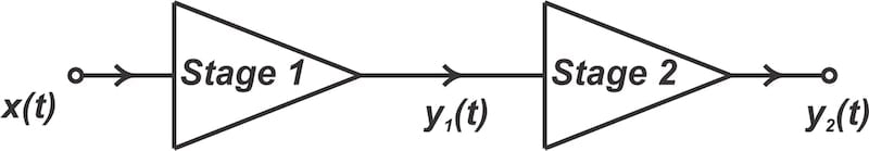
Figure 2. A cascade of two nonlinear stages. Image used courtesy of Steve Arar

 

Assuming that both stages are nonlinear and described by third-degree transfer functions, we have:

$$y_1(t) ~\approx~ \alpha_1 x(t) ~+~ \alpha_2 x^2(t) ~+~ \alpha_3 x^3(t)$$

Equation 3.

 

and:

$$y_2(t) ~\approx~ \beta_1 y_1(t) ~+~ \beta_2 \big (y_1(t) \big)^2 ~+~ \beta_3 \big ( y_1(t) \big )^3$$

Equation 4.

 

We know that all of the frequency components shown in Figure 1 are present at the output of the first stage. Additional distortion components emerge at the final output due to these frequency components passing through the second stage. We won’t find all of these distortion terms here—instead, we’ll explore the mixing mechanisms that result in IM3 components at 2⍵₁ – ⍵₂ and 2⍵₂ – ⍵₁.

The three mechanisms below describe how the nonlinearities of the two stages can generate IM3 components at the output of the second stage.

 

Third-Order Nonlinearity of the First Stage

The third-order term of the first stage (⍺₃) produces the orange components at 2⍵₁ – ⍵₂ and 2⍵₂ – ⍵₁. Upon being applied to the second stage, these components are amplified by the linear term of the second stage (β₁), resulting in new IM3 components at 2⍵₁ – ⍵₂ and 2⍵₂ – ⍵₁ at the second stage’s output.

 

Third-Order Nonlinearity of the Second Stage

The input tones are amplified by the linear term of the first stage (⍺₁), producing the green components in Figure 1. These components then experience the third-order term of the second stage (β₃). As a result, they produce IM3 components at 2⍵₁ – ⍵₂ and 2⍵₂ – ⍵₁ at the final output.

 

Combined Second-Order Nonlinearities of Both Stages

Finally, we know that the second-order nonlinearity of the first stage (⍺₂) produces distortion components at ⍵₂ – ⍵₁, 2⍵₁, and 2⍵₂. Upon experiencing the second-order nonlinearity of the second stage (β₂), these components can produce additional distortion components at 2⍵₁ – ⍵₂ and 2⍵₂ – ⍵₁. For example:

• ⍵₂ – ⍵₁ mixes with ⍵₂ to create a signal at 2⍵₂ – ⍵₁.
• 2⍵₂ mixes with ⍵₁ to also land at 2⍵₂ – ⍵₁.

Therefore, the second-order terms of the two cascaded stages can work together to produce IM3 components. When you think about it, this is kind of interesting!

 

The Phase Relationship Between IM3 Components in a Cascaded System

Based on the above discussion, Figure 3 illustrates the composition of the upper-frequency IM3 product (at 2⍵₂ – ⍵₁).

 

Figure 3. Formation of the upper-frequency IM3 component at 2⍵₂ – ⍵₁. Image used courtesy of Steve Arar

 

Let’s go over each of the color-coded components in this figure. The green component is the result of two distortion mechanisms:

1. The interaction of the first stage’s linear term (⍺₁) with the second stage’s cubic term (β₃)
2. The interaction of the first stage’s cubic term (⍺₃) with the second stage’s linear term (β₁).

The second-order nonlinearity of the second stage causes the second harmonic (2⍵₂) at the output of the first stage to mix with the fundamental component at ⍵₁. This is represented by the orange component. The purple component is produced by the mixing of ⍵₂ – ⍵₁ with ⍵₂, again due to the second-order nonlinearity of the second stage. The vector sum of these three components produces the overall upper-frequency IM3 component at the cascade’s output, which is shown in blue.

The phase relationship between the constituent components of an IM3 product is generally unknown. This means that in the worst-case scenario, these components could align in phase to maximize the IM3 distortion at the output. As the IM3 components are frequently in phase in practical applications, this worst-case approximation effectively mirrors many real-world scenarios.

The reason is that most RF systems have a narrow bandwidth, so the frequency components at ⍵₂ – ⍵₁ and 2⍵₂ fall outside of the circuit’s bandwidth and are heavily suppressed. The remaining frequency components (2⍵₁ – ⍵₂, ⍵₁, ⍵₂, and 2⍵₂ – ⍵₁) are close to each other.

Due to their proximity, these frequencies experience a similar phase shift. As a result, the constituent components of IM3 are commonly in phase. To find the overall IM3 distortion, we simply add them up.

 

Bandwidth-Dependent Nonlinearity in a Single-Transistor Amplifier

Now that we have a better understanding of distortion in cascaded stages, we’re ready to discuss one of the main mechanisms that produces nonlinearity effects in RF PAs. Consider the common-source amplifier in Figure 4, where Z_G is the driving impedance of the stage.

 

Figure 4. A single-transistor amplifier. Image used courtesy of Steve Arar

 

Although this is a single-transistor stage, it’s affected by more than one nonlinearity mechanism. For example, the transistor’s nonlinear parasitic capacitances distort the gate voltage. The drain current is also generated from the gate voltage through another nonlinear relationship. Since this is a simplified model, we can assume that the nonlinearity mechanisms interact similarly to the cascaded stages we previously discussed.

Specifically, the distortion components generated at the gate terminal serve as inputs for the subsequent nonlinearity mechanism. The transistor can therefore be modeled by a cascade of two nonlinear stages. This means that the IM3 component at the amplifier’s output comprises three distinct components, similar to what we saw in Figure 3.

In a typical narrowband RF signal chain, the frequency components that the first stage produces at ⍵₂ – ⍵₁ and 2⍵₂ fall outside of the circuit’s bandwidth and are heavily suppressed. However, with the single-stage amplifier shown in Figure 4, some of these frequency components may see a considerable (and non-constant) impedance at the gate node of the amplifier (node A in Figure 4).

Figure 5 shows the measured gate node impedance for a MESFET amplifier at the baseband, fundamental, and second harmonic frequencies.

 

Figure 5. Measured gate node impedance for a MESFET amplifier at baseband (left), fundamental (middle), and second harmonic (right) frequencies. Image used courtesy of J. Vuolevi

 

While the node impedance is almost constant around the fundamental and second harmonics, it varies considerably at baseband. In the above example, the gate node impedance changes by almost two decades from DC to 20 MHz. Therefore, the attenuation experienced by the frequency component at ⍵₂ – ⍵₁ depends on the frequency separation between the two input tones. For instance, by increasing the frequency separation between the input tones, the component at ⍵₂ – ⍵₁ can experience greater attenuation due to the lowpass impedance of the gate node (left curve in Figure 5).

This suggests that changes in tone spacing affect the output IM3 component, highlighting the bandwidth dependence of dynamic nonlinearity in power amplifiers.

 

Wrapping Up

The previous discussion focused on just one cause of PA nonlinearity effects. There are multiple other mechanisms that contribute to dynamic nonlinearity in PAs, such as dynamic thermal effects and semiconductor trapping phenomena. Thermal effects refer to how the flow and storage of the thermal energy can alter the local, temperature-sensitive properties of the circuit, resulting in a change in PA gain over time. Charge trapping refers to the process in which charge carriers are captured by semiconductor materials and later released, causing dynamic distortion behavior.

Such dynamic deviations from the static characteristics are very troublesome when using predistortion techniques to linearize RF power amplifiers. Understanding each of the underlying causes and addressing them specifically is crucial for eliminating, or at least minimizing, nonlinearity effects in PAs.

 

This article is Part 10 in a series on linearization techniques and nonlinearity in RF systems. Below is a complete list of articles in this series:

1. Introduction to the Feed-Forward Linearization of RF Power Amplifiers
2. Using Analog Predistortion for RF Power Amplifier Linearization
3. Improving RF Power Amplifier Linearity With Digital Predistortion
4. Introduction to the Memory Effect in RF Power Amplifiers
5. Using the 1 dB Compression Point to Characterize RF System Nonlinearity
6. Understanding Intermodulation Distortion and the Third-Order Intercept Point in RF Systems
7. A Guide to Calculating IM3 and IP3 for Nonlinear RF Circuits
8. Understanding Dynamic Range and Spurious-Free Dynamic Range in RF Systems
9. Understanding the Third-Order Intercept Point of a Cascaded System
10. Dynamic Nonlinearity in RF Power Amplifiers: Insights From Two-Tone Testing