Understanding the Third-Order Intercept Point of a Cascaded System

Earlier articles in this series explored key concepts for assessing the linearity of RF components, for example the 1 dB compression point and the third-order intercept point (IP3). In practice, our systems consist of multiple components connected in a cascade arrangement. Ultimately, what we’re interested in is the linearity performance of the whole system.

This article explores the relationship between the linearity of a cascaded system and that of the individual components that constitute the cascade. Understanding this relationship is of paramount importance, as it allows us to identify the components that limit the linearity of the system.

 

Determining the IM3 Component’s Power

With a two-tone input consisting of frequency components at ⍵₁ and ⍵₂, third-order nonlinearity can produce distortion components in the vicinity of the input frequencies. We’ll use the term IM3 to refer to the in-band intermodulation components that appear at 2⍵₁ – ⍵₂ and 2⍵₂ – ⍵₁.

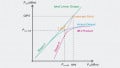
Consider a two-tone test where the power of each input tone is P_1,dBm. Let the powers of the output’s fundamental and IM3 components for this test be, respectively, P_F,dBm and P_IM,dBm, as shown in Figure 1.

 

Figure 1. The powers of the output fundamental and IM3 components vs. the input power in a two-tone measurement.

 

In this portion of the article, we’ll formulate an equation to determine the power of the IM3 component. Later on, we’ll use this equation to assess the nonlinearity of cascaded systems.

Assume that the difference between the applied input power (P_1,dBm) and the input third-order intercept point (IIP_dBm) is ΔP. Since the IM3 power rises with a slope of 3:1, the difference between the output intercept point (OIP_dBm) and P_IM,dBm is 3ΔP. Also, since the slope of the linear output is unity, the difference between OIP_dBm and P_F,dBm is ΔP. As can be seen from the above diagram, the difference between P_F,dBm and P_IM,dBm is 2ΔP:

$$P_{F,dBm} ~-~ P_{IM,dBm} ~=~ 2 ~\times~ \Delta P$$

Equation 1.

 

Substituting OIP_dBm – P_F,dBm = ΔP into the above equation, we obtain:

$$P_{F,dBm} ~-~ P_{IM,dBm} ~=~ 2 ~\times~ \Big (OIP _{dBm} ~-~ P_{F,dBm} \Big )$$

Equation 2.

 

which simplifies to:

$$P_{IM,dBm} ~=~ 3P_{F,dBm} ~-~ 2 OIP _{dBm}$$

Equation 3.

 

In the above analysis, the power quantities are in decibels. The linear equivalent of Equation 3 is:

$$P_{IM} ~=~ \frac{P_{F}^3}{OIP^2}$$

Equation 4.

 

Equation 4, which gives the power quantities in linear terms, stands as the cornerstone of this article. The equation shows that the power of the IM3 component is proportional to the fundamental output power cubed and inversely proportional to the circuit’s output IP3 point squared. Later on, we’ll use this to determine the IM3 component’s power at different nodes of a cascade. Before that, though, we need to examine the mechanisms through which the IM3 component is produced.

 

IM3 Generation in a Cascaded System

Consider a memoryless nonlinear stage whose input-output characteristic is approximated by a third-degree polynomial expression:

$$y(t) ~\approx~ \alpha_0 ~+~ \alpha_1 x(t) ~+~ \alpha_2 x^2(t) ~+~ \alpha_3 x^3(t)$$

Equation 5.

 

If we apply a two-tone input to the above circuit, several different harmonic and non-harmonic (that is, intermodulation) components appear at the output. Figure 2 shows the output frequency components generated in a two-tone test.

 

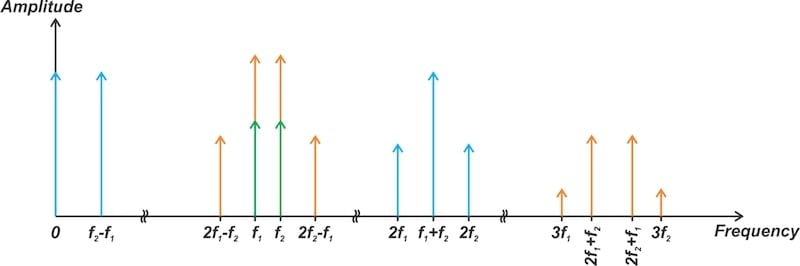
Figure 2. Frequency components produced by the linear term (green), the second-order term (blue), and the third-order term (orange) when the input-output characteristic is modeled by a third-degree expression.

 

Note that the figure does not depict the relative magnitudes of the components, only their presence and the frequencies at which they occur. The relative magnitudes, which depend on the circuit’s nonlinear characteristics, aren’t of concern here.

Next, let’s consider a cascade of two nonlinear stages (Figure 3).

 

Figure 3. A cascade of two nonlinear stages.

 

With a two-tone input, the first stage generates all the frequency components shown in Figure 2 at node A. These frequency components experience the nonlinearity of the second stage and generate the final distortion components at node B. We aim to determine the overall IM3 component that appears at node B.

There are several different distortion components produced by the first stage that can contribute to the IM3 component at the cascade’s output. For instance, Figure 2 shows that the first stage generates a distortion component at 2⍵₂ due to its second-order nonlinearity. This component then mixes with the fundamental component at ⍵₁ due to the second-order distortion of the second stage, producing an intermodulation (IM) product at 2⍵₂ – ⍵₁.

However, it should be noted that the distortion component at 2⍵₂ is far away from the input frequencies (⍵₁ and ⍵₂). Since most RF circuits have a narrow bandwidth, we expect the component at 2⍵₂ to be heavily suppressed by the circuit’s frequency response. Consequently, a simplified nonlinearity analysis of cascaded systems only considers the distortion components in the vicinity of the input frequencies.

With this in mind, let’s examine two mixing mechanisms that produce the output IM3 distortion.

 

Third-Order Nonlinearity of the First Stage

Let’s start with the third-order distortion generated by the first stage. This combines with the linear response of the second stage to produce IM3 components at the output. The relevant frequency components are shown in Figure 4.

 

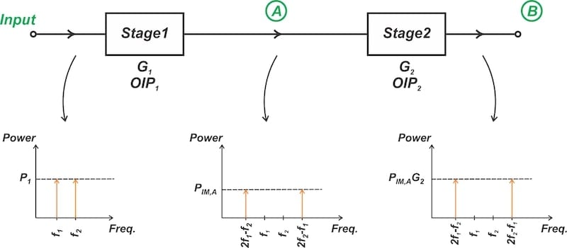
Figure 4. The second stage amplifies the third-order distortion generated by the first stage.

 

In the figure above, we see that the third-order nonlinearity of the first stage produces IM components at frequencies 2⍵₁ – ⍵₂ and 2⍵₂ – ⍵₁ at node A. The second stage amplifies these distortion terms.

We apply Equation 4 to find the power of the IM components at node A, obtaining:

$$P_{IM,A} ~=~ \frac{P_{F,A}^3}{OIP_1^2}$$

Equation 6.

 

where OIP₁ is the output third-order intercept point of the first stage, and P_F,A is the fundamental output power at node A. P_F,A is equal to the input power (P₁) multiplied by the gain of the first stage (G₁):

$$P_{F,A} ~=~ P_1 G_1$$

Equation 7.

 

Combining the previous two equations, we have:

$$P_{IM,A} ~=~ \frac{(P_{1}G_1 ) ^3}{OIP_1^2}$$

Equation 8.

 

The IM power at node A is multiplied by the gain of the second stage (G₂) and appears at the output as:

$$P_{IM,B} ~=~ \frac{(P_{1}G_1 ) ^3 G_2}{OIP_1^2}$$

Equation 9.

 

The above equation determines the contribution of the first mechanism to the output IM3 power.

 

Third-Order Nonlinearity of the Second Stage

The linear gain of the first stage generates fundamental components at the input of the second stage (node A). Due to the third-order nonlinearity of the second stage, they produce third-order IM components at the output (node B). We know from Equation 7 that the fundamental components at node A have a power of P₁G₁. The second stage is therefore excited with a two-tone test where each tone has a power of P₁G₁. This is illustrated in Figure 5.

 

Figure 5. The first stage amplifies the input components and the second stage generates third-order distortion components.

 

Applying Equation 4 to the second stage, we have:

$$P_{IM,B} ~=~ \frac{P_{F,B}^3}{OIP_2^2}$$

Equation 10.

 

In the above equation, OIP₂ is the output third-order intercept point of the second stage and P_F,B is the fundamental output power at node B. P_F,B is equal to the fundamental power input to the second stage (P₁G₁) multiplied by the gain of the second stage (G₂), leading to:

$$P_{IM,B} ~=~ \frac{(P_{1}G_1 G_2 )^3}{OIP_2^2}$$

Equation 11.

 

This is the second mechanism’s contribution to the output IM3 power.

 

Coherent Addition of Distortion Terms

In the previous sections, we calculated the power contributed to the output IM3 component by each stage. The pertinent question is this: how do these constituent components combine to produce the output IM3 distortion?

Since the intermodulation signals are deterministic, we can’t simply add powers. Instead, we have to deal with voltages. We follow a three-step process:

1. Convert the power components into voltages.
2. Add the voltages together to find the total distortion voltage.
3. Convert the result back into a power quantity.

The power from the first mechanism (Equation 9) produces the following distortion voltage:

$$V_1~=~ \sqrt{\frac{(P_{1}G_1 ) ^3 G_2}{OIP_1^2} ~\times~ Z_0}$$

Equation 12.

 

where Z₀ is the system impedance. Similarly, the power from the second mechanism (Equation 11) generates a distortion voltage given by:

$$V_2~=~ \sqrt{\frac{(P_{1}G_1 G_2 )^3}{OIP_2^2} ~\times~ Z_0}$$

Equation 13.

 

In the worst-case scenario, V₁ and V₂ are in-phase and add together to produce the output IM3 voltage:

$$\begin{eqnarray}V_{IM,out} &~=~& V_1 ~+~ V_2 ~=~ \sqrt{\frac{(P_{1}G_1 ) ^3 G_2}{OIP_1^2} ~\times~ Z_0} ~+~ \sqrt{\frac{(P_{1}G_1 G_2 )^3}{OIP_2^2} ~\times~ Z_0} \\&~=~& \sqrt{(P_{1}G_1 G_2 )^3 ~\times~ Z_0} ~\times~ \Big ( \frac{1}{G_2 ~\times~ OIP_1} ~+~ \frac{1}{OIP_2 } \Big )\end{eqnarray}$$

Equation 14.

 

We take the square of V_IM,out and divide the result by Z₀ to find the total output IM3 power:

$$P_{IM,out} ~=~ (P_{1}G_1 G_2 )^3 ~\times~ \Big ( \frac{1}{G_2 \times OIP_1} ~+~ \frac{1}{OIP_2 } \Big )^2$$

Equation 15.

 

Note that the term inside the first parentheses is equal to the fundamental power at the output of the cascade. Denoting this term by P_F,out, we can rewrite the above equation as:

$$P_{IM,out} ~=~ (P_{F,out} )^3 ~\times~ \Big ( \frac{1}{G_2 \times OIP_1} ~+~ \frac{1}{OIP_2 } \Big )^2$$

Equation 16.

 

This equation gives us the IM3 power at the output of the cascade. By noting its resemblance to Equation 4, which describes the IM3 power at the output of a single stage, we can establish an equation for the effective output intercept point of the cascade (OIP_cas):

$$\frac{1}{OIP_{cas}}~=~\frac{1}{OIP_{1}G_2}~+~\frac{1}{OIP_{2}}$$

Equation 17.

 

Intercept Point of a Three-Stage Cascade

Now that we’ve examined the nonlinearity of a two-stage cascade, let’s consider a three-stage cascaded system (Figure 6).

 

Figure 6. A three-stage cascade.

 

We obtain the output intercept point of a three-stage cascade using a similar procedure to the one we used before:

$$\frac{1}{OIP_{cas}}~=~\frac{1}{OIP_{1}G_2 G_3}~+~\frac{1}{OIP_{2}G_3}~+~\frac{1}{OIP_{3}}$$

Equation 18.

 

Note that the denominator terms are simply the intercept points of each stage referred to the output of the entire system. This means that the intercept point of each stage is multiplied by the total gain following that stage. If the total gain of the subsequent stages is relatively large, the fraction associated with that stage becomes relatively small. As a result, the nonlinearity in the final stages of the cascade becomes increasingly critical when the gain terms are substantial.

This can be intuitively understood by noting that the signal amplification by the preceding stages means that the subsequent stages need to deal with relatively larger signals. These larger signals push the later stages in the cascade into more nonlinear regions of operation. The key takeaway is that any nonlinearity present in the later stages will have a more pronounced effect on overall system performance when the gains of the stages are significant.

 

Example: Calculating the Third-Order Intercept Point of a Two-Stage Cascade

To cement what we’ve learned, let’s work through an example problem. Figure 7 shows a low-noise amplifier with an output intercept of +8 dBm and a gain of 13 dB, followed by a mixer that has an input intercept point of 0 dBm and gain of 10 dB.

 

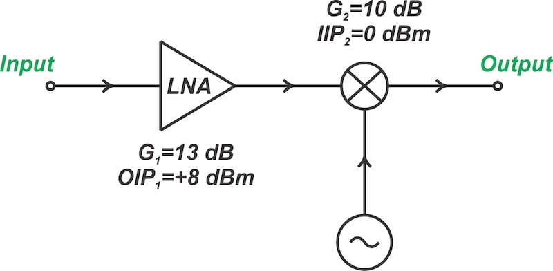
Figure 7. An example of a cascaded system comprising an LNA and mixer.

 

Determine the following for this system:

• The output intercept point of the cascade.
• The input intercept point of the cascade.
• Which stage limits the cascade’s intercept point.

To apply the cascade intercept equation (Equation 17), we first transfer the reference of the mixer’s intercept point from input to the output:

$$OIP_2 ~=~ IIP_2 ~+~ G_2 ~=~ 0 \ \text{dBm} ~+~ 10 \ \text{dB}~=~10 \ \text{dBm}$$

Equation 19.

 

We then convert the decibel values to linear values:

$$\begin{eqnarray} G_1 ~=~ 13 \ \text{dB} \quad &\Rightarrow& \quad G_1~=~10^{1.3}~=~19.95 \\ G_2 ~=~ 10 \ \text{dB} \quad &\Rightarrow& \quad G_2~=~10^{1}~=~10 \\OIP_1 ~=~ 8 \ \text{dBm} \quad &\Rightarrow& \quad OIP_1 ~=~6.3 \ \text{mW} \\ OIP_2 ~=~ 10 \ \text{dBm} \quad &\Rightarrow& \quad OIP_2 ~=~10 \ \text{mW} \end{eqnarray}$$

Equation 20.

 

Substituting these values into Equation 17, we obtain the cascade’s output intercept point:

$$\begin{eqnarray}\frac{1}{OIP_{cas}}&~=~&\frac{1}{OIP_{1}G_2}~+~\frac{1}{OIP_{2}} \\&~=~& \frac{1}{6.3 ~\times~ 10^{-3} ~\times~ 10}~+~\frac{1}{10 ~\times~ 10^{-3}} \\&~=~&115.9\end{eqnarray}$$

Equation 21.

 

From Equation 21, the output intercept point of the cascade works out to OIP_cas = 8.63 mW = 9.4 dBm. The input intercept point of the cascade is equal to the output intercept point minus the total gain in decibels, leading to an input intercept point of 9.4 dBm – (13 + 10) dB = –13.6 dBm.

To determine which stage limits the intercept point of the cascade, let’s assume that the mixer has perfect linearity (OIP₂ = infinity). From the cascade intercept equation, we observe that the system’s output intercept point becomes OIP_cas = OIP₁G₂ as OIP₂ approaches infinity. In this case, using decibel units, OIP_cas works out to 8 dBm + 10 dB = 18 dBm.

This is considerably greater than the output intercept point of the mixer, which is 10 dBm. Therefore, the mixer limits the linearity of the cascade. To verify this, we note that the calculated output intercept point is OIP_cas = 9.4 dBm. This amount is close to the output intercept point of the mixer (OIP₂ = 10 dBm).

 

Wrapping Up

Practical RF systems consist of a cascade of several different blocks. In this article, we discussed how the linearity of the individual constituent stages affects the linearity performance of the cascade as a whole. When the stages have significant gain, any nonlinearity present in the later stages affects the overall system performance more profoundly. For that reason, it’s crucial to carefully manage and understand the nonlinearity in the final stages, especially when dealing with substantial gains.

 

This article is Part 9 in a series on linearization techniques and nonlinearity in RF systems. Below is a complete list of articles in this series:

1. Introduction to the Feed-Forward Linearization of RF Power Amplifiers
2. Using Analog Predistortion for RF Power Amplifier Linearization
3. Improving RF Power Amplifier Linearity With Digital Predistortion
4. Introduction to the Memory Effect in RF Power Amplifiers
5. Using the 1 dB Compression Point to Characterize RF System Nonlinearity
6. Understanding Intermodulation Distortion and the Third-Order Intercept Point in RF Systems
7. A Guide to Calculating IM3 and IP3 for Nonlinear RF Circuits
8. Understanding Dynamic Range and Spurious-Free Dynamic Range in RF Systems
9. Understanding the Third-Order Intercept Point of a Cascaded System
10. Dynamic Nonlinearity in RF Power Amplifiers: Insights From Two-Tone Testing

 

All images used courtesy of Steve Arar