A Guide to Calculating IM3 and IP3 for Nonlinear RF Circuits

In the intricate world of RF systems, understanding and managing intermodulation distortion is essential for achieving the desired performance. With a two-tone input consisting of frequency components at ⍵₁ and ⍵₂, third-order nonlinearity can produce distortion components in the vicinity of the input frequencies. These distortion products, which appear at 2⍵₁ – ⍵₂ and 2⍵₂ – ⍵₁, are referred to as IM3 components.

IM3 components are of particular interest to us, as they’re likely to interfere with the desired signals and degrade the performance of the system. To quantify them, we use the third-order intercept point (IP3) metric. The IP3 point is defined as the hypothetical intercept point of the power curves of the fundamental and IM3 components.

As well as possessing a keen understanding of intermodulation distortion, RF engineers should be capable of estimating the power of IM3 components and the IP3 point of RF circuits. To help you hone these capabilities, this article presents a series of example problems and explains their solutions.

 

Overview of Basic Concepts

As we know from earlier articles in this series, we commonly use a third-degree polynomial expression to model the input-output characteristic of a memoryless, nonlinear circuit. Denoting the circuit’s output by y(t), we have:

$$y(t) ~\approx~ \alpha_0 ~+~ \alpha_1 x(t) ~+~ \alpha_2 x^2(t) ~+~ \alpha_3 x^3(t)$$

Equation 1.

 

where x(t) is a two-tone input comprising frequency components at ⍵₁ and ⍵₂:

$$x(t) ~=~ A \cos(\omega_1 t) ~+~ A \cos(\omega_2 t)$$

Equation 2.

 

This input causes the circuit to generate several different distortion components at the output. Assuming that the circuit is only weakly nonlinear, the amplitudes of the fundamental components experience a gain of ⍺₁ from the input to the output, whereas the IM3 components that emerge at 2⍵₁ – ⍵₂ and 2⍵₂ – ⍵₁ have an amplitude of 3⍺₃A³/4. This is illustrated in Figure 1.

 

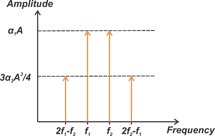
Figure 1. The IM3 components at 2f₁ – f₂ and 2f₂– f₁.

 

The preceding article also introduced us to two metrics used to quantify intermodulation distortion:

• The intermodulation distortion ratio (IMR), which is defined as the ratio of the amplitude of one of the intermodulation terms to the amplitude of the desired output signal.
• The third-order intercept point (IP3), which represents the hypothetical intersection of the power curves for the fundamental frequency and IM3 components.

In this case, the IMR is:

$$IMR ~=~ \frac{\frac{3}{4} \alpha_3 A^3}{\alpha_1 A}~=~ \frac{3}{4} \frac{\alpha_3}{\alpha_1} A^2$$

Equation 3.

 

The definition of the IP3 point is illustrated in Figure 2.

 

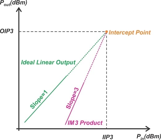
Figure 2. Illustration of the third-order intercept point.

 

It can be shown that the input amplitude corresponding to the IP3 point is given by:

$$A_{IP} ~=~ \sqrt{\frac{4}{3}\frac{\alpha_1}{\alpha_3}}$$

Equation 4.

 

Estimating the IP3 Point from a Single Measurement

Typically, determining the IP3 point involves extrapolation from the results of multiple measurements performed in the amplifier’s linear region of operation. However, for a preliminary approximation of the IP3 point, the outcome of a single test may suffice. In this case, we apply a two-tone input with signal levels well below the amplifier’s compression point and measure the powers of the fundamental and IM3 output components.

In Figure 3, both input tones have a power of P₁. The powers of the output’s fundamental and IM3 components are denoted by P_F and P_IM3, respectively.

 

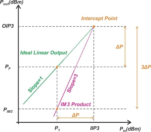
Figure 3. Estimating the IP3 point from a single measurement.

 

Let’s use P₁, P_F, and P_IM3 to determine the input IP3 point of the amplifier. Assume that the difference between the applied input power (P₁) and the IIP3 point is ΔP.

Since the IM3 power rises with a slope of 3:1, the difference between OIP3 and P_IM3 is 3ΔP. By the same token, since the slope of the linear output is unity, the difference between OIP3 and P_F is ΔP. Finally, as we can see in the above diagram, the difference between P_F and P_IM3 is 2ΔP. We therefore have:

$$P_F ~-~ P_{IM3} ~=~ 2 \Delta P ~=~ 2 ~\times~ (IIP3 ~-~ P_1)$$

Equation 5.

 

Rearranging this equation, we obtain:

$$IIP3 ~=~ P_1 ~+~ \frac{1}{2} (P_F ~-~ P_{IM3})$$

Equation 6.

 

Example 1: Determining IIP3 from a Single Measurement

Consider an amplifier designed to operate at 2 GHz with a gain of 10 dB. An input consisting of two equal-amplitude tones at 2 GHz and 2.01 GHz is applied to the amplifier. Given the output frequencies and power levels provided in Table 1, estimate the IIP3 of the amplifier.

 

Table 1. Output frequencies and powers for Example 1.

Output Frequency (GHz)	Output Power (dBm)
1.99	–75
2.00	–25
2.01	–25
2.02	–75

 

Figure 4 shows the output frequency components.

 

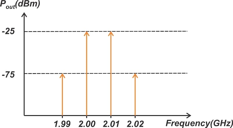
Figure 4. The frequency components at the amplifier’s output.

 

The frequency components at 2 GHz and 2.01 GHz are the fundamental output components. Since these components exhibit a power level of –25 dBm and the amplifier’s gain is 10 dB, the input tones have a power of P₁ = –35 dBm. We can now calculate the IIP3 by substituting P_F = –25 dBm and P_IM3= –75 dBm into Equation 5:

$$IIP3 ~=~ P_1 ~+~ \frac{1}{2} (P_F ~-~ P_{IM3})~=~-35 ~+~ \frac{1}{2} ~\times~ \big ( -25 ~-~ (-75) \big )~=~-10~ \text{dBm}$$

Equation 7.

 

According to Equation 7, the IIP3 works out to –10 dBm.

 

Example 2: Finding IM3 Components With a Two-Tone Input at a Given Power Level

Consider an amplifier with an input third intercept point of IIP3 = +20 dBm. We apply an input consisting of two tones with equal amplitudes to the amplifier. If each tone has a power of 0 dBm, how many decibels less is the IM3 component than the fundamental component? Assume that interface impedances are 50 Ω.

We’ll explore two different ways of solving this example. The first one is relatively complex, whereas the second uses a more intuitive approach.

 

The Mathematical Approach

First, let’s use the following equation to convert the IIP3 power value from dBm to mW:

$$P(mW) ~=~ 10^{(\frac{P(dBm)}{10})}$$

Equation 8.

 

According to Equation 8, an IIP3 of +20 dBm translates to an input power of 100 mW. Assuming 50 Ω interfaces, an IIP3 of 100 mW corresponds to a signal amplitude of 3.16 V, as calculated below:

$$P ~=~ \frac{1}{2} \frac{A_{IP}^2}{R} \quad \Rightarrow \quad 0.1 ~=~ \frac{1}{2} \frac{A_{IP}^2}{50} \quad \Rightarrow \quad A_{IP}~=~3.16~ \text{V}$$

Equation 9.

 

As in Equation 4, A_IP denotes the input voltage amplitude of the IP3 point. By rearranging Equation 4, we get:

$$\frac{\alpha_1}{\alpha_3} ~=~ \frac{3}{4} \big( A_{IP} \big)^2$$

Equation 10.

 

Substituting A_IP = 3.16 V into the above equation, we obtain:

$$\frac{\alpha_1}{\alpha_3}~=~7.49 ~\text{V}^2$$

Equation 11.

 

Recall that the IMR specification gives the amplitude of the IM3 component normalized to the fundamental component:

$$IMR ~=~ \frac{\frac{3}{4} \alpha_3 A^3}{\alpha_1 A}~=~ \frac{3}{4} \frac{\alpha_3}{\alpha_1} A^2$$

Equation 12.

 

where A is the input signal amplitude.

We calculated the ratio of ⍺₁ to ⍺₃ in Equation 11. We only need to determine the input signal amplitude that corresponds to a power value of 0 dBm.

From Equation 8, 0 dBm is equal to 1 mW. With 50 Ω interfaces, a power of 1 mW represents a signal amplitude of A = 0.316 V. Substituting these values into Equation 12, we obtain:

$$IMR ~=~ \frac{3}{4} ~\times~ 7.49^{-1} ~\times~ 0.316^2 ~=~0.01 ~=~ -40 ~\text{dB}$$

Equation 13.

 

With 0 dBm input tones, the amplitude of the IM3 components is one-hundredth of that of the fundamental components. Equivalently, the IM3 component is 40 dB less than the carrier. You may also see this denoted as dBc to emphasize the calculation of decibels with respect to the carrier.

 

The Graphical Approach

An easier way of solving this problem is to note how the fundamental and IM3 components change with the input power level. Consider the diagram in Figure 5.

 

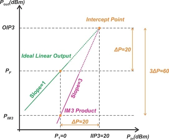
Figure 5. Graphical representation of the information in Example 2.

 

We know that the power curves corresponding to the fundamental and IM3 components have, respectively, a slope of 1:1 and 3:1. These two lines also pass through the IIP3 point at +20 dBm. An input power of 0 dBm corresponds to a power change of ΔP = 20 dBm on the horizontal axis.

Considering the slopes of the lines, the power of the fundamental component (P_F) is ΔP = 20 dBm less than the OIP3, whereas the power of the IM3 component (P_IM3) is 3ΔP = 60 dBm below the OIP3. At an input power of 0 dBm, the power of the IM3 component is therefore 2ΔP = 40 dBm less than that of the fundamental component.

 

Example 3: Finding Fundamental and IM3 Components at a Given Input Power Level

Consider an amplifier with a gain of 10 dB. We apply an input consisting of two equal-amplitude tones to the amplifier where each input tone has a power of –15 dBm. In this case, the IM3 component is –60 dBm. Determine the fundamental and IM3 powers for a two-tone test where each tone has a power of –20 dBm.

This example, like the previous one, can be easily solved through the graphical method. Figure 6 illustrates the information given in the problem.

 

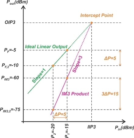
Figure 6. Graphical representation of Example 3.

 

We calculate the fundamental and IM3 components by reducing the input power from –15 dBm (P₁) to –20 dBm (P₂) on the horizontal axis. This corresponds to a power change of ΔP = 5 dBm, with the following results.

1. Because the fundamental component has a slope of 1:1, the fundamental output power changes by ΔP = 5 dBm: from –5 dBm (P_F) to –10 dBm (P_F,2).
2. Because the IM3 product has a slope of 3:1, the output power of the IM3 component changes by 3ΔP = 15 dBm: from –60 dBm (P_IM3) to –75 dBm (P_IM3,2).

At an input power of –20 dBm, the power of the fundamental and IM3 components are therefore –10 dBm and –75 dBm, respectively.

 

Final Takeaway: An Unsolved Example

To solidify your understanding and put your skills to the test, I've included an unsolved example directly drawn from “RF Microelectronics” by B. Razavi as an exercise for you:

 

A low-noise amplifier senses a –80 dBm signal at 2.410 GHz and two –20 dBm interferers at 2.420 GHz and 2.430 GHz. What IIP3 is required if the IM3 products must remain 20 dB below the signal? For simplicity, assume 50 Ω interfaces at the input and output.

 

I hope that you’ve found the solved examples in this article helpful, and that engaging with this final problem enhances your grasp of the concepts we’ve discussed.

 

This article is Part 7 in a series on linearization techniques and nonlinearity in RF systems. Below is a complete list of articles in this series:

1. Introduction to the Feed-Forward Linearization of RF Power Amplifiers
2. Using Analog Predistortion for RF Power Amplifier Linearization
3. Improving RF Power Amplifier Linearity With Digital Predistortion
4. Introduction to the Memory Effect in RF Power Amplifiers
5. Using the 1 dB Compression Point to Characterize RF System Nonlinearity
6. Understanding Intermodulation Distortion and the Third-Order Intercept Point in RF Systems
7. A Guide to Calculating IM3 and IP3 for Nonlinear RF Circuits
8. Understanding Dynamic Range and Spurious-Free Dynamic Range in RF Systems
9. Understanding the Third-Order Intercept Point of a Cascaded System
10. Dynamic Nonlinearity in RF Power Amplifiers: Insights From Two-Tone Testing

 

All images used courtesy of Steve Arar