Improving RF Power Amplifier Linearity With Digital Predistortion

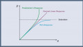
To maximize efficiency, power amplifiers (PAs) are operated over a large dynamic range that edges towards the saturation region. As we approach the saturation region, amplitude and phase distortions increase remarkably, resulting in significant adjacent channel interference.

Several different linearization techniques have been developed to enhance the linearity of RF PAs while maintaining their high efficiency. In this article, we'll learn about one of the most active areas in RF power amplifier linearization: digital predistortion. As we'll see, the digital approach allows for the creation of complex predistortion transfer characteristics that surpass the capabilities of the basic analog methods we discussed previously.

Basics of Digital Predistortion

Digital predistortion compensates the PA's nonlinearity by introducing a nonlinear function in the digital portion of the transmit path, as illustrated in Figure 1. Either the baseband or intermediate frequency signal is altered.

Figure 1. Realizing digital predistortion in baseband.

Though the basic schematic in the above figure depicts an open-loop predistortion system, we commonly incorporate a feedback path to continuously monitor the predistorter's performance and adjust it accordingly. Figure 2 shows the simplified block diagram of a digital predistortion linearizer with a feedback loop.

Figure 2. Digital predistortion system with feedback path.

Using feedback enables adaptive digital predistortion systems that can account for temperature, process, or voltage variations. However, the analog-to-digital converters (ADCs), DSP, and memory increase total power consumption. This extra power use results in decreased system efficiency, as we'll discuss in the next section.

Calculating the Efficiency of the Predistorter/PA System

Consider the following scenario: an adaptive digital predistortion system employs a PA with 100% efficiency and an output power of 1 W. Accompanying this setup, the predistortion system components—including the ADCs, DSP, and memory units—collectively require 0.25 W of power. Given these conditions, let's determine the total efficiency of the combined predistorter/PA system.

The efficiency is equal to the ratio of the output power to the total power drawn from the supply (\(\eta~=~\frac{P_L}{P_{cc}}\)). The supply power is equal to the output power plus power dissipated by the system components (\(P_{cc}~=~P_L~+~P_{dissipated}\)). Therefore, we have:

$$\eta ~=~ \frac{P_L}{P_{cc}} ~=~ \frac{P_L}{P_L ~+~ P_{dissipated}}~=~\frac{1}{1~+~0.25}~=~80 \%$$

Equation 1.

Although the PA has an efficiency of 100%, the power consumption of the associated circuits brings the system's overall efficiency down to 80%. For that reason, it's important to keep the linearizer's power consumption as small as possible compared to the PA's output power.

Digital Predistortion Using Look-Up Tables

If the PA behavior is quasi-static, we can assume that the PA's output amplitude has a fixed, monotonic relationship to the input signal. In this scenario, the output signal's value is solely determined by the present input value. Consequently, it's possible to determine the PA's nonlinear behavior.

Encoding this data into a look-up table (LUT) gives us several options for implementing a digital predistortion system. Figure 3 illustrates one of them.

Figure 3. Block diagram of an open-loop, LUT-based predistortion system.

The input signal is used to address the PA distortion look-up table, which holds the necessary gain and phase correction values (Δ|A| and Δφ, respectively) for each input value. The DSP block receives Δ|A| and Δφ and produces an amplitude and phase-adjusted signal that ensures the predistorter/PA system operates linearly.

Like Figure 1, the above predistortion linearizer is an open-loop system. Figure 4 shows an LUT-based system that incorporates a feedback loop to monitor the linearization integrity and update the look-up table accordingly.

Figure 4. An adaptive, LUT-based predistortion system.

The adaptive system shown above includes both a transmitter (forward path) and an integrated receiver (reverse path). The adaptation block compares the input I/Q signal to the I/Q sample obtained from the integrated receiver. This enables the system to assess the efficacy of the predistortion mechanism and refresh the data within the look-up table accordingly.

The feedback loop of the predistorter operates very slowly and doesn't need to adjust to rapid changes. For that reason, this adaptive predistorter doesn't suffer from the stability issues that are typically associated with feedback linearization methods.

The look-up table typically implements either a mapping predistortion function or a complex-gain predistortion function. As we'll discuss shortly, the former employs cartesian mapping, whereas the latter relies on envelope mapping. The LUT function directly influences the size and complexity of the utilized look-up table.

Mapping Predistortion

The mapping predistorter offers a straightforward but brute-force strategy for indexing the look-up table. Figure 5 illustrates the application of the LUT within this methodology.

Figure 5. The look-up table indexing method used in the mapping predistorter circuit.

The mapping predistorter uses a pair of two-dimensional look-up tables (LUT-I and LUT-Q in the figure above). In this context, “two-dimensional” signifies that both in-phase (I_IN) and quadrature (Q_IN) signals are used to index the look-up tables. The tables' outputs are therefore a function of both the in-phase and quadrature signals. Each point of the I/Q complex plane is mapped to a new value.

Mapping predistortion can correct any errors associated with the upconversion process, including the DC offsets and I/Q imbalance. However, the memory requirements of this technique present a significant drawback. Because it re-maps each input point to a corresponding new value, the mapping predistorter needs a large memory. Noting that both I_IN and Q_IN components together serve as the indices for the table's entries, the total number of memory entries (M) is given by:

$$M~=~2~\times~2^{2n}$$

Equation 2.

where n is the number of bits used for quantizing the amplitude of the I_IN and Q_IN signals. For instance, a 12-bit system necessitates a memory with M = 33,554,432 entries.

Completing the adaptation algorithm requires processing every point on the I/Q complex plane, which takes a substantial amount of time. For this reason, a large memory results in long adaptation times and increased computational complexity.

Complex-Gain Predistortion

As its name suggests, the complex gain technique stores complex-valued gain factors in a look-up table. Figure 6 illustrates the application of the LUT within a complex-gain predistorter.

Figure 6. The LUT indexing method used in the complex-gain predistorter.

In this method, the power of the input signal (\(R~=~|I_{IN}~+~jQ_{IN}|\)) is used to point to a memory entry with the appropriate gain factor. The complex-gain technique ensures that the combined predistorter and PA system maintains a constant gain at all output power levels.

Since the input signal envelope serves as the index for the table's entries, a smaller look-up table is required. This also reduces the power consumption associated with both interpolation and adaptation. However, these improvements come at the price of diminished predistortion accuracy, which restricts the effective suppression of intermodulation distortion.

Wrapping Up

Digital predistortion is among the most effective methods of RF power amplifier linearization. In this article, we discussed two digital predistortion techniques: mapping predistortion and complex-gain predistortion.

As we learned, the primary limitation of the mapping predistorter lies in its substantial memory requirements. These requirements lead to long adaptation times and increased computational complexity. The complex-gain predistorter is often favored over the mapping predistorter technique, as it requires a smaller look-up table and reduces the adaptation time.

This article is Part 3 in a series on linearization techniques and nonlinearity in RF systems. Below is a complete list of articles in this series:

1. Introduction to the Feed-Forward Linearization of RF Power Amplifiers
2. Using Analog Predistortion for RF Power Amplifier Linearization
3. Improving RF Power Amplifier Linearity With Digital Predistortion
4. Introduction to the Memory Effect in RF Power Amplifiers
5. Using the 1 dB Compression Point to Characterize RF System Nonlinearity
6. Understanding Intermodulation Distortion and the Third-Order Intercept Point in RF Systems
7. A Guide to Calculating IM3 and IP3 for Nonlinear RF Circuits
8. Understanding Dynamic Range and Spurious-Free Dynamic Range in RF Systems
9. Understanding the Third-Order Intercept Point of a Cascaded System
10. Dynamic Nonlinearity in RF Power Amplifiers: Insights From Two-Tone Testing

All images used courtesy of Steve Arar