Understanding Intermodulation Distortion and the Third-Order Intercept Point In RF Systems

Learn how the two-tone input test helps us evaluate the nonlinearity of RF systems operating on real-world signals.

Technical Article May 28, 2025 by Dr. Steve Arar

In the previous article of this series, we delved into how nonlinear systems respond to a single-tone input. When a single frequency is applied to a nonlinear system, harmonic components at integer multiples of this frequency appear at the output. These harmonic components may lie outside of the passband of the amplifier, causing them to be heavily attenuated. In this case, the single-tone test may overstate how linear the circuit actually is.

Because practical circuits process input signals consisting of many frequencies, a two-tone test with two closely-spaced frequencies produces a more realistic assessment of the circuit’s nonlinearity. It also allows us to examine the intermodulation products, which are what we call distortion components that aren’t harmonics of the input frequencies. Even if the circuit has a very narrow bandwidth, the small frequency separation between the input tones allows us to generate distortion components that lie within the passband of the circuit.

In this article, we’ll use a two-tone input test to examine intermodulation distortion in a memoryless, nonlinear system. We’ll also learn about the third-order intercept point (IP3), an essential metric for characterizing this form of nonlinearity.

Distortion Components Produced by A Two-Tone Input

Figure 1 shows a device or network with input x(t) and output y(t). We’ll assume that this device is both nonlinear and memoryless.

A general device or network.

Figure 1. A general device or network.

Let’s examine this system’s response to the following two-tone input, which comprises frequency components at ⍵₁ and ⍵₂:

$$x(t) ~=~ A_1 \cos(\omega_1 t) ~+~A_2 \cos(\omega_2 t)$$

Equation 1.

For simplicity, we’ll assume that both tones have an amplitude of A.

If the circuit is memoryless, we can use a polynomial expression to approximate its input-output characteristic:

$$y(t) ~\approx~ \alpha_0 ~+~ \alpha_1 x(t) ~+~ \alpha_2 x^2(t) ~+~ \alpha_3 x^3(t) ~+~ \alpha_4 x^4(t)~+~...$$

Equation 2.

The term ⍺₁ in the polynomial expression represents the linear coefficient, which amplifies the input signal without distorting it. Denoting this part of the output signal by y₁(t), we have:

$$y_1(t) ~=~ \alpha_1 A \big ( \cos(\omega_1 t) ~+~ \cos(\omega_2 t) \big )$$

Equation 3.

We commonly retain terms up to and including the third-order in the polynomial expression, a practice we’ll maintain in this article.

The Second-Order Term

The second-order term, which is represented by the coefficient ⍺₂, produces an output voltage of:

$$\begin{eqnarray}y_2(t) &~=~& \alpha_2 A^2 \big ( \cos(\omega_1 t) ~+~ \cos(\omega_2 t) \big )^2 \\&~=~& \alpha_2 A^2 \Big (1~+~ \frac{1}{2} \cos(2 \omega_1 t)~+~\frac{1}{2} \cos(2 \omega_2 t)~+~\cos \big( (\omega_1 ~+~ \omega_2)t \big )~+~\cos \big( (\omega_1 ~-~ \omega_2)t \big ) \Big )\end{eqnarray}$$

Equation 4.

From Equation 4, we observe that the second-order term produces energy at the following frequencies:

DC.
The second harmonic of the input tones (2⍵₁ and 2⍵₂).
The difference frequency (|(⍵₁ – ⍵₂|).
The sum frequency (⍵₁ + ⍵₂).

Figure 2 shows the frequency components produced by the second-order term. For simplicity, only the positive frequencies are shown.

Distortion products generated by the second-order term.

Figure 2. Distortion products generated by the second-order term.

Figure 2 confirms that the circuit generates intermodulation products—distortion components that aren’t harmonics of the input frequencies—with a two-tone input.

Note that the spectrum of a cosine term such as Acos(⍵t) consists of two impulses, one at ⍵ and one at –⍵. Each has an amplitude of A/2. Despite being excited with signals at f₁ and f₂, the output spectrum of a circuit with second-order nonlinearity doesn’t have any signal components at these frequencies.

The Third-Order Term

Next, let’s examine the intermodulation products generated by the third-order term:

$$\begin{eqnarray}y_3(t) &~=~& \alpha_3 A^3 \big ( \cos(\omega_1 t) ~+~ \cos(\omega_2 t) \big )^3 \\&~=~& \frac{9}{4}\alpha_3 A^3 \Big (\cos( \omega_1 t)~+~ \cos(\omega_2 t) \Big ) \\ && ~+~ \frac{1}{4}\alpha_3 A^3 \Big (\cos(3 \omega_1 t)~+~ \cos(3 \omega_2 t) \Big ) \\&& ~+~ \frac{3}{4} \alpha_3 A^3 \Big ( \cos \big( (2\omega_1 ~+~ \omega_2)t \big )~+~\cos \big( (2\omega_1 ~-~ \omega_2)t \big ) \Big ) \\&& ~+~ \frac{3}{4} \alpha_3 A^3 \Big ( \cos \big( (2\omega_2 ~+~ \omega_1)t \big )~+~\cos \big( (2\omega_2 ~-~ \omega_1)t \big ) \Big )\end{eqnarray}$$

Equation 5.

The third-order term produces energy at the fundamental frequencies (⍵₁ and ⍵₂), at the third harmonics (3⍵₁ and 3⍵₂), at 2⍵₁ ± ⍵₂, and at 2⍵₂ ± ⍵₁. These frequency components are shown in Figure 3.

Figure 3. Distortion components generated by the third-order nonlinearity.

The third-order distortion doesn’t generate energy at the frequencies where the second-order distortion components are present.

The Full Range of Distortion Products

Figure 4 combines Figures 2 and 3 to obtain the complete range of distortion products produced by the third-degree expression.

Frequency components produced by the linear term (green), the second-order term (blue), and the third-order term (orange) when the input-output characteristic is modeled by a third-degree expression.

Figure 4. Frequency components produced by the linear term (green), the second-order term (blue), and the third-order term (orange) when the input-output characteristic is modeled by a third-degree expression.

Note that this figure is meant only to show the presence of different components and the frequencies at which they occur. The relative magnitudes of the components, which depend on the nonlinear characteristics of the circuit, aren’t of concern here.

Before we move on, it’s worth mentioning that we can assign an order to each distortion product of the form m⍵₁ + n⍵₂, where the order is defined as |m| + |n|. By this definition, the intermodulation products at 2⍵₁, 2⍵₂, ⍵₂ – ⍵₁, and ⍵₁ + ⍵₂ are all of the second order.

Narrowband Systems Can Suppress Distortion Components

As shown in Figure 4, a third-degree nonlinear characteristic produces several different distortion products. These range from DC up to the third harmonics. Such distortion components can be heavily suppressed if they’re sufficiently outside of the circuit’s passband.

This is particularly important in RF circuits with a narrow bandwidth. If the circuit has a narrow bandwidth around the fundamental components, the distortion products at all of the following frequencies will be attenuated by the circuit’s bandpass response:

Difference terms: ⍵₂ – ⍵₁
Sum term: ⍵₁ + ⍵₂
Harmonic terms: 2⍵₁, 2⍵₂, 3⍵₁, 3⍵₂
Intermodulation terms: 2⍵₁ + ⍵₂,2⍵₂ + ⍵₁

Attenuation of the out-of-band distortion components can make the circuit appear more linear than it actually is. However, an input signal consisting of two closely-spaced frequencies can generate in-band distortion components even if the circuit has a very narrow bandwidth. Determining these distortion terms allows us to assess the linearity of the circuit.

As we saw in Figure 4, the distortion components at 2⍵₁ – ⍵₂ and 2⍵₂ – ⍵₁ are very close in frequency to the fundamental components (⍵₁ and ⍵₂). These intermodulation products, which we’ll refer to as IM3 components in the rest of the article, are of particular interest to us.

Intermodulation Distortion Metrics

Consider three Bluetooth devices transmitting at f₁ = 2.41 GHz, f₂ = 2.42 GHz, and f₃ = 2.43 GHz, respectively. Noting that 2f₂ – f₃ = 2.41 GHz, we observe that the signals sent out at 2.42 GHz and 2.43 GHz can generate an IM3 component for a receiver device operating at 2.41 GHz.

These IM3 components pose a significant challenge in RF systems. Having a method to quantify this effect, so that we can assess and compare the linearity across various systems, is essential. One metric is the intermodulation distortion ratio (IMR), which is defined as the ratio of the amplitude of one of the intermodulation terms to the amplitude of the desired output signal:

$$IMR ~=~ \frac{\frac{3}{4} \alpha_3 A^3}{\alpha_1 A}~=~ \frac{3}{4} \frac{\alpha_3}{\alpha_1} A^2$$

Equation 6.

An important limitation of this linearity metric is that it varies with the signal level. When comparing systems, we ideally want a metric that’s only a function of the circuit parameters. To get around this issue, we use the third-order intercept point (IP3) metric instead.

Consider Figure 5, which shows how the powers of the fundamental output and the IM3 component change with the input power.

The third-order intercept point.

Figure 5. The third-order intercept point.

While the fundamental component exhibits a slope of 1:1, the IM3 components rise 3 dB for every 1 dB increase in the input power. This is because the fundamental output component is proportional to A, whereas the IM3 products are proportional to A³ (see Equation 5).

Even though the IM3 components are very small at low input powers, they grow rapidly with the input amplitude due to their cubic dependence on A. Therefore, if we keep increasing the input power, there should theoretically be a point where the powers of the fundamental and IM3 products become equal.

This is what we refer to as the third-order intercept point. In the above figure, it’s marked in orange. The input power and output power at the intercept point are denoted by IIP3 and OIP3, respectively.

Determining the IP3 Point

In practice, both the fundamental and the IM3 components exhibit compression at high input powers, as illustrated in Figure 6.

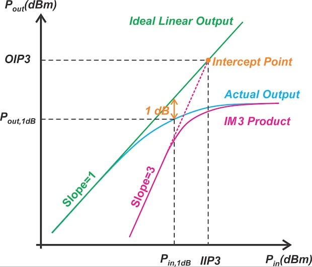
Third-order intercept point for systems with gain compression.

Figure 6. Third-order intercept point for a system with gain compression.

The IP3 can’t be measured directly. Instead, it’s obtained by extrapolating the fundamental and IM3 power curves from their linear operation regions and finding the intercept point. As mentioned above, this is the point at which the amplitude of the IM3 component becomes equal to the amplitude of the fundamental output component. By applying this definition, we can establish a relationship between the signal amplitude at the IP3 point and the coefficients of the third-order polynomial approximation.

From Equation 5, the amplitude of the IM3 component is:

$$A_{IM3} ~=~\frac{3}{4} \alpha_3 A^3$$

Equation 7.

Meanwhile, the amplitude of the fundamental output component is:

$$A_{fund} ~=~ \alpha_1 A$$

Equation 8.

If we set A_IM3 equal to A_fund and solve for A, we obtain the input amplitude (A_IP) corresponding to the IP3 point:

$$A_{IP} ~=~ \sqrt{\frac{4}{3}\frac{\alpha_1}{\alpha_3}}$$

Equation 9.

If we know the coefficients ⍺₁ and ⍺₃, we can use the above equation to determine the input signal amplitude corresponding to the IP3 point.

Wrapping Up

In this article, we examined what happens when a two-tone input is applied to a memoryless, nonlinear system. When we represented this system using a polynomial approximation, we saw that the input frequency components are mixed (multiplied) by the higher-order polynomial terms. This generates intermodulation distortion (IM3) components at frequencies that are not harmonics of the inputs. We focused on the third-order distortion terms at 2⍵₁ – ⍵₂ and 2⍵₂ – ⍵₁, as these are typically very close in frequency to the fundamental components at ⍵₁ and ⍵₂.

To quantify the IM3 components, we use the third-order intercept point (IP3) metric. The IP3 point is a measure of the system’s nonlinearity. It allows us to assess the ability of the system to receive a weak signal in the presence of large-amplitude interferers that are close in frequency to the desired signal.

This article is Part 6 in a series on linearization techniques and nonlinearity in RF systems. Below is a complete list of articles in this series: