Using the 1 dB Compression Point to Characterize RF System Nonlinearity

Multiple mechanisms contribute to nonlinearity in electronic systems. For example, the transconductance of active devices is influenced by the signal amplitude. The parasitic capacitances and resistances within these devices are also amplitude-dependent, which can affect the circuit's performance. Furthermore, surpassing the circuit’s normal signal swing even briefly can result in the clipping of signal troughs or peaks, introducing substantial nonlinearity into the system.

At high power levels, all practical components exhibit nonlinearity. In RF circuits, this can result in increased losses, signal distortion, and possible interference with other radio channels. Nonlinearity can be characterized in several ways, each one of which offers a unique perspective on how a circuit deviates from linear behavior under different conditions.

In this article, we’ll delve into two forms of RF circuit nonlinearity: harmonic distortion and gain compression. We’ll also explore the 1 dB compression point, a useful metric for characterizing gain compression.

 

What is the 1 dB Compression Point?

As illustrated in Figure 1, the 1 dB compression point is defined as the power level at which output power falls 1 dB below the ideal linear characteristic. We use this specification to quantify the upper limit of an RF circuit’s linear operation.

 

Figure 1. The 1 dB compression point is used as a metric for quantifying the circuit’s linearity.

 

The 1 dB compression point can be expressed in terms of either the input or output power:

$$P_{out, 1db} ~=~ P_{in, 1dB} ~+~ (G_p ~-~ 1)$$

Equation 1.

 

where:

G_p is the ideal linear gain of the amplifier in decibels

P_in,1dB is the input power at which compression occurs

P_out,1dB is the output power at which compression occurs.

For amplifiers, the 1 dB compression point is usually specified as the output power at which compression occurs. For mixers, it’s usually stated in terms of the input power corresponding to the compression point. The input compression point of RF receivers is typically in the range of –20 to –25 dBm.

Now that we know what the 1 dB compression point is, let’s take a step back and consider the behavior of nonlinear systems more generally. This discussion will lay the groundwork for us to understand harmonic distortion and gain compression. We’ll return to the 1 dB compression point later on.

 

Modeling a Memoryless Nonlinear System

Consider a device or system with input x(t) and output y(t), as shown in Figure 2.

 

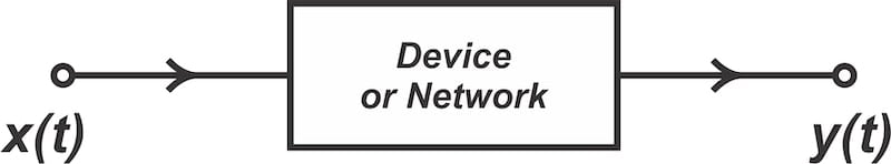
Figure 2. A generic device or network.

 

The network is linear and memoryless if its transfer characteristic is:

$$y(t) ~=~ \alpha_1 x(t)$$

Equation 2.

 

where ⍺₁ is a constant independent of time. If the above condition isn’t satisfied, the circuit is nonlinear. The input-output characteristics of memoryless nonlinear systems can be approximated by a polynomial expression:

$$y(t) ~\approx~ \alpha_0 ~+~ \alpha_1 x(t) ~+~ \alpha_2 x^2(t) ~+~ \alpha_3 x^3(t) ~+~ \alpha_4 x^4(t)~+~...$$

Equation 3.

 

We commonly retain terms up to and including the third-order in the polynomial expression, leading to:

$$y(t) ~\approx~ \alpha_0 ~+~ \alpha_1 x(t) ~+~ \alpha_2 x^2(t) ~+~ \alpha_3 x^3(t)$$

Equation 4.

 

Observe that in the above equations, the output's instantaneous value at any given time (t) is solely determined by the input's value at that same moment. This condition defines a memoryless characteristic. If the output at time t is influenced by previous input values, the characteristic is said to exhibit the memory effect.

In systems with memory, time-delayed inputs or their derivatives and integrals may appear in the output equation. For example, the output signal could be a function that depends on x(t) in the following manner:

$$y(t) ~=~ g \Big [x(t), \ \int_{- \infty}^{t} x(t) dt, \ \frac{d^n x(t)}{dt^n} \Big ]$$

Equation 5.

 

Harmonic Distortion

The nonlinear properties of the polynomial approximations can be examined for either a single-tone or a two-tone input. Let’s see what happens if we apply the following single-tone input to the nonlinear characteristic of Equation 4:

$$x(t) ~=~ A_1 cos(\omega_1 t)$$

Equation 6.

 

We obtain:

$$y(t) ~\approx~ \alpha_0 ~+~ \alpha_1 A_1 \cos(\omega_1 t) ~+~ \alpha_2 \big ( A_1 \cos(\omega_1 t) \big ) ^2 ~+~ \alpha_3 \big ( A_1 \cos(\omega_1 t) \big ) ^3$$

Equation 7.

 

The second-order term produces an output signal of:

$$y_2(t) ~=~ \alpha_2 \big ( A_1 cos(\omega_1 t) \big ) ^2 ~=~ \frac{1}{2} \alpha_2 A_1^2 \big (1 ~+~ cos(2 \omega_1 t) \big )$$

Equation 8.

 

The second-order nonlinearity generates frequency components at both DC and the second harmonic (2⍵₁).

On the other hand, the third-order term produces:

$$y_3(t) ~=~ \alpha_3 \big ( A_1 \cos(\omega_1 t) \big ) ^3 ~=~ \frac{1}{4} \alpha_3 A_1^3 \big (3 \cos(\omega_1 t) ~+~ \cos(3 \omega_1 t) \big )$$

Equation 9.

 

The third-order term generates frequency components at both the fundamental frequency and the third harmonic (3⍵₁).

Combining Equations 7, 8 and 9, the total output signal for a third-degree transfer function is:

$$y(t) ~=~ \alpha_0 ~+~ \frac{1}{2} \alpha_2 A_1^2 ~+~ \big ( \alpha_1 A_1 ~+~ \frac{3}{4} \alpha_3 A_1^3 \big ) \ \cos(\omega_1 t) ~+~ \frac{1}{2} \alpha_2 A_1^2 \ \cos(2 \omega_1 t)~+~ \frac{1}{4} \alpha_3 A_1^3 \ \cos(3 \omega_1 t)$$

Equation 10.

 

With the single-tone input at ⍵₁, the higher-order terms of the equation produce frequency components at all harmonics of the input. This phenomenon is referred to as harmonic distortion.

 

Output Power at Different Harmonics

Let’s assume that x(t) and y(t) in the above discussion are voltage quantities. From Equation 10, the amplitude of the fundamental voltage component is:

$$v_{o,fund} ~=~ \alpha_1 A_1 ~+~ \frac{3}{4} \alpha_3 A_1^3$$

Equation 11.

 

The total output signal at ⍵₁ comprises two distinct terms: the linear term and the third-order term. For low levels of input power, the linear term is dominant. We’ll ignore the third-order term for now.

With resistances normalized to unity, the output power at the fundamental frequency is:

$$P_{fund} ~=~ 10 \log \big (\frac{1}{2} \frac{v_{o,fund}^2}{R} \big ) ~=~ 10 \log \big ( \frac{1}{2} \alpha_1^2 A_1^2 \big ) ~=~ 20 \log(\alpha_1)~+~ 10 \log \big ( \frac{1}{2} A_1^2 \big )$$

Equation 12.

 

The last term in the above equation is the power of the input signal:

$$P_{fund} ~=~ 20 \log(\alpha_1)~+~ P_{in}$$

Equation 13.

 

This means that, for low input power values, the fundamental output power rises by 1 dB for every 1 dB increment in input power.

What about the second and third harmonic components? From Equation 10, the output power at the second harmonic is:

$$\begin{eqnarray}P_{2} &~=~& 10 \log \big (\frac{1}{2} \frac{v_{o,2}^2}{R} \big ) ~=~ 10 \log \Big ( \frac{1}{2} ~\times~ (\frac{1}{2} \alpha_2 A_1^2)^2 \Big ) \\&~=~& 10 \log \big ( \frac{\alpha_2^2}{2} \big) ~+~ 2 ~\times~ 10 \log ( \frac{1}{2} A_1^2) \\&~=~& 10 \log \big ( \frac{\alpha_2^2}{2} \big) ~+~ 2 P_{in} \end{eqnarray}$$

Equation 14.

 

Therefore, the output power at the second harmonic rises by 2 dB for every 1 dB increase in the input power. Similarly, it can be shown that for the third harmonic, the slope of the output power versus input power curve is 3:1. In general, the power level of the nth harmonic exhibits a slope of n:1 when the powers are expressed in decibels. This is illustrated in Figure 3.

 

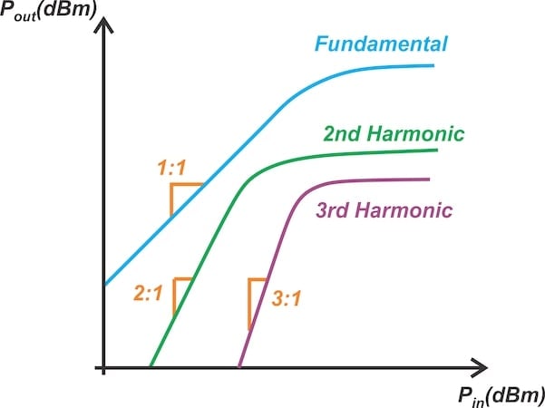
Figure 3. Output power vs. input power at different harmonics.

 

In the weakly nonlinear region, the power of the fundamental frequency increases by 1 dB for each 1 dB increase in the input power. The second and third harmonics rise by 2 dB and 3 dB, respectively.

For a practical circuit operating beyond the weakly nonlinear region, the power in the harmonic frequencies may not increase monotonically with respect to the input power. This is due to the influence of the higher-order nonlinearity terms that were neglected in our third-degree polynomial expression.

 

Gain Compression

At higher input powers, the output begins to saturate. This means the output power no longer increases linearly with the input power. One reason is that the power supply voltage limits the circuit’s maximum output voltage.

Figure 3 shows that the amplifier’s gain at the fundamental frequency is dependent on the input power and drops off as the input power increases. To better understand this, let’s use Equation 10 to determine the gain at the fundamental frequency:

$$G ~=~\frac{Output \ at \ \omega_1}{Input \ at \ \omega_1}~=~\frac{\alpha_1 A_1 ~+~ \frac{3}{4} \alpha_3 A_1^3}{A_1}~=~\alpha_1 ~+~ \frac{3}{4} \alpha_3 A_1^2$$

Equation 15.

 

At low input powers, the term ⍺₁ dominates, making the gain equal to the small-signal gain of the amplifier. However, as the input signal amplitude increases, the second term in the above equation grows rapidly.

For most practical circuits, ⍺₁ and ⍺₃ have opposite signs. Consequently, there is a decrease in gain at higher power levels. This phenomenon is known as gain compression.

 

Determining the 1 dB Compression Point

Using the 1 dB compression point as a metric, we can determine the signal amplitude at which compression occurs in terms of the coefficients of the polynomial expression. Applying the definition given at the beginning of the article, the actual gain of the amplifier given by Equation 15 is 1 dB below the ideal gain (⍺₁) at the compression point. We therefore have:

$$20 \log (|\alpha_1|) ~-~ 20 \log \big ( |\alpha_1 ~+~ \frac{3}{4} \alpha_3 A_1^2|)~=~1$$

Equation 16.

 

which simplifies to:

$$\Big |\frac{\alpha_1 ~+~ \frac{3}{4} \alpha_3 A_1^2}{\alpha_1} \Big|~=~10^{-1/20} ~\approx~ 0.891$$

Equation 17.

 

Finally, we obtain:

$$A_1 ~=~ 0.38 \sqrt{|\frac{\alpha_1}{\alpha_3}|}$$

Equation 18.

 

This is the input signal amplitude at which 1 dB compression occurs.

 

Key Takeaways

Even with a single-tone input, a nonlinear circuit generates outputs at integer multiples of the input frequency. This phenomenon is referred to as harmonic distortion.

Furthermore, with a single-tone input, the total output signal of a nonlinear circuit at the fundamental frequency is made up of a linear term and a third-order nonlinear term. In practical circuits, this produces gain compression.

To quantify the upper limit of the circuit’s linear region, we use the 1 dB compression point. This is defined as the power level at which the output power falls 1 dB below the ideal linear characteristic.

 

This article is Part 5 in a series on linearization techniques and nonlinearity in RF systems. Below is a complete list of articles in this series:

1. Introduction to the Feed-Forward Linearization of RF Power Amplifiers
2. Using Analog Predistortion for RF Power Amplifier Linearization
3. Improving RF Power Amplifier Linearity With Digital Predistortion
4. Introduction to the Memory Effect in RF Power Amplifiers
5. Using the 1 dB Compression Point to Characterize RF System Nonlinearity
6. Understanding Intermodulation Distortion and the Third-Order Intercept Point in RF Systems
7. A Guide to Calculating IM3 and IP3 for Nonlinear RF Circuits
8. Understanding Dynamic Range and Spurious-Free Dynamic Range in RF Systems
9. Understanding the Third-Order Intercept Point of a Cascaded System
10. Dynamic Nonlinearity in RF Power Amplifiers: Insights From Two-Tone Testing

 

All images used courtesy of Steve Arar